Chapter 10: Catalysis and Catalytic Reactors
Topics
- Octane Rating
- Steps in Catalytical Reaction
- Rate Limiting Step
- Regulation for Automotive Exhaust Emissions
- Chemical Vapor Deposition
- Types of Catalyst Deactivation
- Temperature-Time Trajectories
- Moving Bed Reactors & Straight Through Transport Reactors
Octane Rating
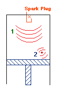
TopA Typical Engine Piston
|
|
|
Determine the compression ratio, CR, The more compact molecules are (for a given |
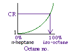 100% isooctane = 100 octane number 100% heptane = 0 octane number |

|
English |
|
| Espanol | |
| Svenska |
Molecular Adsorption
\(\text{H}_2 + S \rightleftharpoons \text{H}_2 \cdot S\)
At equilibrium:
\(r_{AD} = 0 = k \left[ P_{\text{H}_2} C_V - \frac{C_{\text{H}_2 \cdot S}}{K_{\text{H}_2}} \right]\)
\(C_{\text{H}_2 \cdot S} = K_{\text{H}_2} P_{\text{H}_2} C_V\)
\(C_t = C_V + C_{\text{H}_2 \cdot S}\)
\(C_{\text{H}_2 \cdot S} = \frac{K_{\text{H}_2} P_{\text{H}_2}}{1 + K_{\text{H}_2} P_{\text{H}_2}} C_t\)
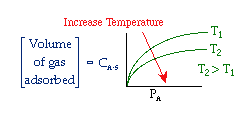
Langmuir Isotherms
|
Dissociative Adsorption
\(\text{H}_2 + 2S \rightleftharpoons 2\text{H} \cdot S\)
At equilibrium:
\(r_{AD} = 0 = k \left[ P_{\text{H}_2} C_V^2 - \frac{C_{\text{H}_2 \cdot S}^2}{K_H} \right]\)
\(C_{\text{H} \cdot S} = C_T \frac{\sqrt{P_{\text{H}_2} K_H}}{1 + \sqrt{P_{\text{H}_2} K_H}}\)
Steps in a Catalytic Reaction
Top|
\( A \leftrightarrow B \) |
|||
|
Adsorption on Surface |
\( A + S \leftrightarrow A \bullet S \) |
||
|
Surface Reaction |
Single Site |
\( A \bullet S \leftrightarrow B \bullet S \) |
|
|
Dual Site |
\( A \bullet S + S \leftrightarrow B \bullet S + S \) |
||
|
Desorption from Surface |
\( B \bullet S \leftrightarrow B + S \) |
||
|
\( A + B \leftrightarrow C + D \) |
||
|
Adsorption on Surface |
\( A + S \leftrightarrow A \bullet S \) |
|
|
\( B + S \leftrightarrow B \bullet S \) |
||
|
Surface Reaction |
Dual Site |
\( A \bullet S + B \bullet S \leftrightarrow C \bullet S + D \bullet S \) |
|
\( A \bullet S + B \bullet S' \leftrightarrow C \bullet S + D \bullet S' \) |
||
|
Eley-Rideal |
\( A \bullet S + B (g) \leftrightarrow C \bullet S + D (g) \) |
|
|
Desorption from Surface |
\( C \bullet S \leftrightarrow C + S \) |
|
|
\( D \bullet S \leftrightarrow D + S \) |
||
Example: Catalytic Reaction to Improve the Octane Number of Gasoline
|
\( \text{n-pentane} \leftrightarrow \text{i-pentane} \) \( \text{75% Pt} \) \( \text{on } \text{Al}_2\text{O}_3 \) |
||
|
Rationale: |
n-pentane: Octane No. = 62 |
|
|
The difference in octane ratings provides |
||
|
Steps in this reaction: |
||
|
\( \text{n-pentane} \overset{\text{Pt}, -H_2}{\leftrightarrow} \text{n-pentene} \overset{\text{Al}_2O_3}{\leftrightarrow} \text{i-pentene} \overset{\text{Pt}, +H_2}{\leftrightarrow} \text{i-pentane} \) |
||
|
Focusing on the second reaction: |
||
|
\( \text{n-pentene} \leftrightarrow \text{i-pentene} \) \( \text{Al}_2O_3 \) \( N \leftrightarrow I \) |
||
Rate Limiting Steps
Top|
Adsorption |
\( N + S \leftrightarrow N \bullet S \) |
\( r_{AD} = k_A \left[ P_N C_{\vee} - \frac{C_{N \bullet S}}{K_N} \right] \) |
|
Surface Reaction |
\( N \bullet S \leftrightarrow I \bullet S \) |
\( r_S = k_S \left[ C_{N \bullet S} - \frac{C_{I \bullet S}}{K_S} \right] \) |
|
Desorption |
\( I \bullet S \leftrightarrow I + S \) |
\( r_D = k_D \left[ C_{I \bullet S} - \frac{P_I C_{\vee}}{K_{DI}} \right] = k_D \left[ C_{I \bullet S} - K_R P_I C_{\vee} \right] \) |
|
Assume surface reaction is rate limiting |
\( -r_S = k_S \left[ C_{N S} - \frac{C_{I \bullet S}}{K_S} \right] \) |
|
|
If the surface reaction is limiting then: |
||
|
\( \frac{r_{AD}}{k_A} \approx 0 \quad \therefore \quad C_{N \bullet S} = K_N P_N C_{\vee} \) |
see also stirctly speaking link |
|
\( \frac{r_D}{k_D} \approx 0 \quad \therefore \quad C_{I \bullet S} = K_I P_I C_{\vee} \) |
see also strictly speaking link |
|
|
\( -r_N = k_S \left[ K_N P_N - K_I P_I \right] C_{\vee} = k_S K_N \left[ P_N - \frac{P_I}{K_P} \right] C_{\vee} \) \( \text{where } K_P = \frac{K_S K_N}{K_I} \) |
||
|
Site balance: |
\( C_T = C_{\vee} + C_{N \bullet S} + C_{I \bullet S} \) |
|
|
Substituting for CN-S, CI-S, and CV into CT = CV (1 + KN PN + KI PI) : |
||
|
\( -r_N' = \frac{k_S K_N C_T \left[ P_N - \frac{P_I}{K_P} \right]}{1 + K_N P_N + K_I P_I} \) |
||
|
where KP is the thermodynamic equilibrium constant for the reactor. |
||
|
Linearizing the Initial Rate: |
||
|
\( -r_N' = \frac{k P_{N0}}{1 + K_N P_{N0}} \quad \Rightarrow \quad \frac{P_{N0}}{-r_N'} = \frac{1}{k} + \frac{K_N}{k} P_{N0} \) 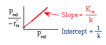
|
| Single Site | |||
|---|---|---|---|
| A) |
\( A \cdot S \rightarrow B \cdot S \) |
\(-r'_A = \frac{k P_A}{1 + K_A P_A + K_B P_B} \) |
Plot |
| Dual Site | |||
| B) |
\( A \cdot S + S \rightarrow B \cdot S + S \) |
\(-r'_A = \frac{k P_A}{(1 + K_A P_A + K_B P_B)^2} \) |
Plot |
| C) |
\( A \cdot S + B \cdot S \rightarrow C \cdot S + S \) |
\(-r'_A = \frac{k P_A P_B}{(1 + K_A P_A + K_B P_B + K_C P_C)^2} \) |
Plot |
| Eley-Rideal | |||
| D) |
\( A \cdot S + B(g) \rightarrow C \cdot S \) |
\(-r'_A = \frac{k P_A P_B}{1 + K_A P_A + K_C P_C} \) |
Plot |
|
\( 2CO + O_2 \mathrel{\substack{\xrightarrow{} \\ \xleftarrow{\text{cat}}}} 2CO_2 \) |
Regulations for Automotive Exhaust Emissions
Top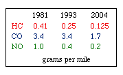
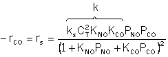
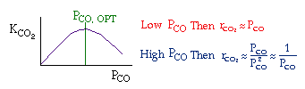
Example
| Let's see what fraction of sites are covered by CO at the optimum: | |
|
\( K_{CO} P_{CO} = 1 + K_{NO} F_{NO} \) |
|
| Multiplying by CV: | |
|
\( C_{\vee} K_{CO} P_{CO} = C_{\vee} + C_{\vee} K_{NO} P_{NO} \) |
|
| (A) |
\( C_{CO \bullet S} = C_{\vee} + C_{NO \bullet S} \) |
| (B) |
\( C_t = C_{\vee} + C_{NO \bullet S} + C_{CO \bullet S} \) |
|
\( \frac{C_{CO \bullet S}}{C_t} = \frac{1}{2} \) |
|
Chemical Vapor Deposition
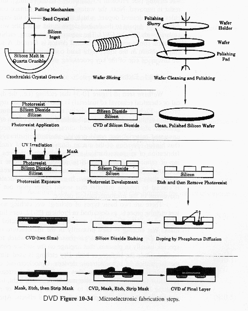
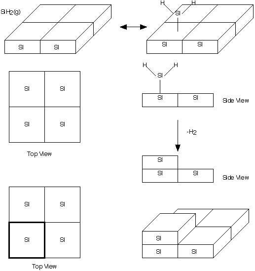
TopManufacturing of a Silicon Layer
|
We see that a number of the key steps in the microelectronic
fabrication involve CVD, we shall consider the CVD of silicon.
| I Mechanism | ||
| (1) \( \text{SiH}_4 (g) \leftrightarrow \text{SiH}_2 (g) + \text{H}_2 (g) \) |
\( -\tilde{r}_{\text{SiH}_4} = k_g \left[ P_{\text{SiH}_4} - P_{\text{SiH}_2} P_{\text{H}_2} / K_P \right] \) |
|
| (2) \( \text{SiH}_2 (g) + S \leftrightarrow \text{SiH}_2 \bullet S \) |
\( r_{AD} = k_A \left[ P_{\text{SiH}_2} f_v - \frac{f_{\text{SiH}_2}}{K_{\text{SiH}_2}} \right] \) |
|
| (3) \( \text{SiH}_2 \bullet S \rightarrow \text{Si} + \text{H}_2 (g) \) |
\( r_S = k_S f_{\text{SiH}_2} \) |
|
|
||
| II Rate Limiting Step (Reaction 3) | ||
| \( r_{\text{dep}} = r_S = k_S f_{\text{SiH}_2} \) | ||
| III Expressing fSiH2 in Terms of Partial Pressures | ||
| \( \frac{r_{AD}}{k_A} \approx 0 \quad \Rightarrow \quad f_{\text{SiH}_2} = K_{\text{SiH}_2} P_{\text{SiH}_2} f_v \) | ||
| \( -\tilde{r}_{\text{SiH}_2} = r_S = k_S f_{\text{SiH}_2} = k_S K_{\text{SiH}_2} P_{\text{SiH}_2} f_v \) | ||
| IV Site / Surface Area Balance: | ||
|
\( f_{\text{SiH}_2} + f_v = 1 \quad \Rightarrow \quad K_{\text{SiH}_2} P_{\text{SiH}_2} f_v + f_v = 1 \) \( f_v = \frac{1}{1 + K_{\text{SiH}_2} P_{\text{SiH}_2}} \) |
||
|
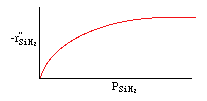
\[ -\tilde{r}_{\text{SiH}_2} = k_S K_{\text{SiH}_2} \frac{P_{\text{SiH}_2}}{1 + K_{\text{SiH}_2} P_{\text{SiH}_2}} \] |
|
|
Types of Catalyst Deactivation
Top| Separable Kinetics: | \( -\dot{r}_A(t) = a(t) \left[ -\dot{r}_A(\text{fresh catalyst}) \right] \) |
Types of Decay
Temperature-Time Trajectories
TopThe catalyst decay rate is a function of temperature, so you can vary the temperature with time to keep the rate of decay as constant as possible.
| \( -r_A(T_0,\, t = 0) = r_A(T, t) \) | |
| Then: | |
|
\( k_o = a(t) \, k(T) \) \( t = \frac{1 - \exp \left[ \frac{E_A - n E_A + E_d}{R} \left( \frac{1}{T} - \frac{1}{T_0} \right) \right]} {k_{40} \left( 1 - n + \frac{E_d}{E_A} \right)} \) |
|
| or solving for \( T = f(t) \) | |
| \( T = \frac{(E_A - n E_A + E_d) T_0} {(E_A - n E_A + E_d) - R T_0 \ln \left[ \frac{1}{1 - k_D t \left( 1 - n + \frac{E_d}{E_A} \right)} \right]} \) |
Moving Bed Reactors & Straight Through Transport Reactors
TopCatalyst Decay Example
The gas-phase, irreversible reaction
\( \text{A} \xrightarrow{\text{cat}} \text{B} \) is
elementary
with first order decay. The reaction is carried out at constant temperature and
pressure.
| Parameters | Batch Reactor | Moving Bed Reactor | Straight Through Transport Reactor |
|---|---|---|---|
| Mole Balance |
\(\frac{dX}{dt} = \frac{-r_A W}{N_{A0}}\) |
\(\frac{dX}{dW} = \frac{-r_A}{F_{A0}}\) |
\(\frac{dX}{dz} = \frac{-r_A}{F_{A0}}\) |
| Rate Law |
\(-r_A = a(t)kC_A\) |
\(-r_A = a(t)kC_A\) |
\(-r_A = \rho_B a(t)kC_A\) |
| Decay Law |
\(-\frac{da}{dt} = k_D a\) \(a = e^{-k_D t}\) |
\(W = U_s t\) \(-\frac{da}{dW} = \frac{k_D}{U_s} a\) \(a = e^{-\frac{k_D W}{U_s}}\) |
\(z = U_p t\) \(-\frac{da}{dz} = \frac{k_D}{U_p} a\) \(a = e^{-\frac{k_D z}{U_p}}\) |
| Stoichiometry |
\(C_A = C_{A0}(1 - X)\) |
\(C_A = C_{A0}(1 - X)\) |
\(C_A = C_{A0}(1 - X)\) |
| Combine |
\(\frac{dX}{dt} = \frac{e^{-k_D t} k W C_{A0}(1 - X)}{N_{A0}}\) \(N_{A0} = C_{A0} v = C_{A0} \frac{W}{\rho_B}\) \(\frac{dX}{dt} = k \rho_B e^{-k_D t}(1 - X)\) \(\frac{dX}{1 - X} = k \rho_B e^{-k_D t} dt\) \(\ln{\frac{1}{1 - X}} = \frac{k \rho_B}{k_D} \left[ 1 - e^{-k_D t} \right]\) |
\(\frac{dX}{dW} = \frac{e^{-\frac{k_D W}{U_s}} k C_{A0}(1 - X)}{F_{A0}}\) \(F_{A0} = C_{A0} v_0\) \(\frac{dX}{1 - X} = \frac{k}{v_0} e^{-\frac{k_D W}{U_s}} dW\) \(\ln{\frac{1}{1 - X}} = \frac{k U_s}{v_0 k_D} \left[ 1 - e^{-\frac{k_D W}{U_s}} \right]\) |
\(\frac{dX}{dz} = \frac{\rho_B a k C_{A0}(1 - X)}{F_{A0}}\) \(F_{A0} = C_{A0} v_0 A_C\) \(\frac{dX}{1 - X} = \frac{\rho_B k}{v_0} e^{-\frac{k_D z}{U_p}} dz\) \(\ln{\frac{1}{1 - X}} = \frac{\rho_B U_p k}{v_0 k_D} \left[ 1 - e^{-\frac{k_D z}{U_p}} \right]\) |
Gas phase, but \(\delta = 0\), \(T = T_0\), and \(P = P_0\)
Another Catalyst Decay Example
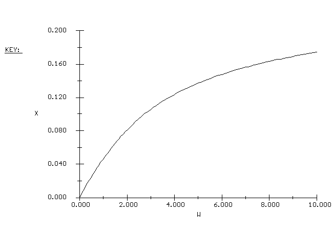
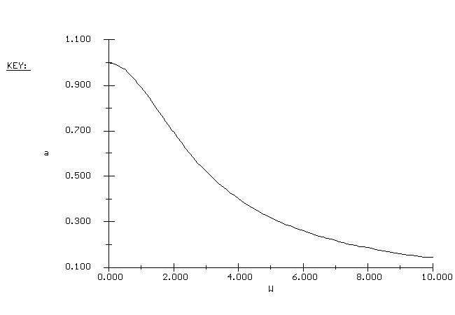
The second-order, irreversible reaction \( \text{A} \xrightarrow{\text{cat}} \text{B} \) is carried out in a moving bed reactor. The catalyst loading rate is 1 kg/s to a reactor containg 10 kg of catalyst. The rate of decay is second order in activity and first order in concentration for the product, B, which poisons the catalyst. Plot the conversion and activity as a function of catalyst weight down the reactor.
Additional information:
\( C_{A0} = 0.1 \; \text{mol/dm}^3 \) \( \nu_0 = 10 \; \text{dm}^3/\text{mol/s} \)
\( k_D = 50 \; \text{dm}^3/\text{mol/s} \) \( k_R = 50 \; \text{dm}^6/(\text{mol} \cdot \text{kg} \cdot \text{s}) \)
Solution:
| Polymath | ||
|---|---|---|
| Mole Balance: | \( \frac{dX}{dW} = \frac{-r_A}{F_{A0}} \) | |
| Rate Law: | \( -r_A = a(t) \, k_R \, C_A^2 \) | |
| Decay Law: | \( -\frac{da}{dt} = k_D \, a^2 \, C_B \) | |
| \( W = U_S \, t \) | ||
| \( -\frac{da}{dW} = \frac{k_D}{U_S} \, a^2 \, C_B \) | ||
| Stoichiometry: | \( C_A = C_{A0} (1 - X) \) | |
| \( C_B = C_{A0} \, X \) | ||
| Combine: | \( \frac{dX}{dW} = a \left( \frac{k_R C_{A0}^2}{F_{A0}} \right) (1 - X)^2 = a \, k_{1R} (1 - X)^2 \) | |
| \( \frac{da}{dW} = -\left( \frac{k_D C_{A0}}{U_S} \right) a^2 X = -k_{2D} a^2 X \) | ||
| \( k_{1R} = \frac{k_R C_{A0}^2}{F_{A0}} = \frac{(50)(0.1)^2}{10} = 0.05 \; \text{kg}^{-1} \) | ||
| \( k_{2D} = \frac{k_D C_{A0}}{U_S} = \frac{(50)(0.1)}{1} = 5.0 \; \text{kg}^{-1} \) | ||
| Conversion vs. Catalyst Weight |
 |
| Catalyst Activity vs. Catalyst Weight |
 |
Example 10-7: Strictly Speaking
| When there is a change in the velocity due to a change in the number of moles up through the STTR, one cannot directly substitute t = z/U in the coking activity equation: | ||
|
\( a = \frac{1}{1 + A t^{1/2}} \) |
(1) | |
| Instead, one must add another equation to the Polymath program. We know that at any location, the gas velocity up the column is: | ||
|
\( \frac{dz}{dt} = U \) |
(2) | |
| Then: | ||
|
\( \frac{dt}{dz} = \frac{1}{U} \) |
(3) | |
| where t = 0 at z = 0. You can use either Polymath or MatLab to solve this equation and substitute it for t in the activity equation: |
||
|
\( a = \frac{1}{1 + A t^{1/2}} \) |
||
| Along with: | ||
|
\( \frac{dX}{dz} = \frac{-r_A}{U \, C_{A0}} \) |
||
|
\( \frac{dt}{dz} = \frac{1}{U} \) |
||
|
\( U = U_0 (1 + \varepsilon X) \) |
||
| etc.
(same as the program in Table E10-7.1) |
||
* All chapter references are for the 4th Edition of the text Elements of Chemical Reaction Engineering .