Chapter 10: Catalysis and Catalytic Reactors
Catalyst Decay in a Packed Bed
The reaction
\( 3 \, \text{H}_2 + \text{CO} \rightarrow \text{CH}_4 + \text{H}_2\text{O} \)
is carried out with excess H2 in a long packed-bed reactor containing a Ni–Mo–Cu catalyst. The reaction is first order in CO. The rate of catalyst decay is first order in CO and first order in the catalytic activity. The exiting carbon monoxide concentration was monitored as a function of time in two separate experiments, one at a high volumetric flow rate and one at a low volumetric flow rate.
For a space time of 1.0 h:
| t (h) | 1 | 4 | 8 | 12 | 16 | 20 | 24 |
|---|---|---|---|---|---|---|---|
| CO (mol/dm³) × 10² | 0.05 | 0.11 | 0.30 | 0.58 | 0.82 | 0.93 | 0.98 |
For a space time of 100 h:
| t (h) | 10 | 500 | 1000 | 1050 | 1090 | 1095 | 1100 | 1090 | 1095 | 1100 |
|---|---|---|---|---|---|---|---|---|---|---|
| CO (mol/dm³) × 10² | 0 | 0 | 0 | 0 | 0.047 | 0.18 | 0.50 | 0.95 | 0.99 | 1.0 |
Expectations
Initially the reactor is filled with inert gas and at time t = 0 the reactant gas mixture is fed to the reactor. At the start, the reactant gas sees only fresh catalyst and methane is produced. As time goes on the catalyst at front of the reactor becomes spent as a result of being poisoned by CO and the entering reactant gas must travel further down the reactor to reach fresh catalyst.
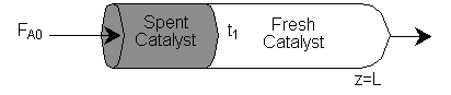
As time continues, the activity front moves on down the reactor and eventually breaks through the end of the reactor at time called the break through time tb. The figure below shows the activity profile down the reactor as a function of time. The activity profile shown is relatively steep, but the steepness will be a function of the reaction rate and the flow rate.
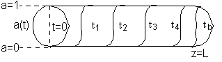
Activity Profile as a function of time.
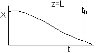
If one were to look at the exit, (z = L) the conversion of CO, it might look something like
either
 or
or 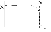
(a) (b)
(a) or (b) depending on the rate of reaction and the Damköhler number. We note that same phenomena occurs in similar systems such as the leaching of uranium, the acidization of petroleum wells, and in chromatographic reactors.
Analysis
Packed bed reactor with catalyst decay
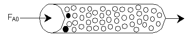
\( 3 \, \text{H}_2 + \text{CO} \xrightarrow{\text{Ni-Mo-Cu}} \text{CH}_4 + \text{H}_2\text{O} \)
Assumptions
(1) Neglect volume change because of XS H2 (yA0 << 1 \ e @ 0)
(2) Neglect pressure drop
(3) Neglect axial dispersion
(4) Neglect CO, consumed to Poison sites
A. The Algorithm
\( F_A \Big|_z - F_A \Big|_{z+\Delta z} + \vec{r_A} \rho_b \frac{\pi D^2}{4} \Delta z = \frac{\pi D^2}{4} \Delta z \frac{\partial C_A}{\partial t} \)
\( F_A = C_A \nu = C_A U \frac{\pi D^2}{4} \)
Mole Balance
\( \frac{\partial C_A}{\partial t} + U \frac{\partial C_A}{\partial z} - r_A = 0 \)
Rate Law
\( -r_A = a k C_A \quad \text{Note: } -r_A = \rho_b \left( -r_A' \right) = a \rho_b k C_A \)
Decay Law
\( \frac{\partial a}{\partial t} \Big|_z = -k_d a C_A \)
Stoichiometry
Gas phase
\( U = U_0 \, (\epsilon \sim 0) \)
\( \Delta P = 0, \quad \Delta T = 0 \)
Combine
\( \frac{\partial C_A}{\partial t} + U \frac{\partial C_A}{\partial z} + k_a C_A = 0 \)
\( \frac{\partial a}{\partial t} = -k_d C_A \)
Initially, there is an inert gas in the reactor and at time t = 0 we will begin feeding the fresh reactant gas.
| IC | t = 0 | CA = 0 | z > 0 | ||
| BC | z > Ut | a = ao | (ao = 1) | ||
| z = 0 | t > 0 | CA = CA0 |
B. Putting the Equations in Dimensionless Form
Let
\( \psi = \frac{C_A}{C_{A0}} , \quad \eta = \frac{a}{a_0} , \quad \epsilon = \frac{z}{L} \)
\( \tau = \frac{V}{v} = \frac{L}{U} , \quad \theta = \frac{t}{\tau} \)
\( \frac{\partial \psi}{\partial \epsilon} + \frac{\partial \psi}{\partial \sigma} + k \cdot r_a \cdot \eta \cdot \psi = 0 \)
\( \frac{\partial \psi}{\partial \epsilon} + \frac{\partial \psi}{\partial \sigma} + Da \cdot \eta \cdot \psi = 0 \)
Da = Damköhler number which gives the shape of decay front = \( = k \cdot r_a \cdot a_0 \)
\( D_a = k r_{a0} = \frac{k C_{A0} a_0 V}{C_{A0} \nu_0} = -\frac{r_{A0} V a_0}{F_{A0}} = \frac{\text{rate of reaction of A}}{\text{rate of transport of A by convection}} \)
\( \left( \frac{\partial \eta}{\partial \varepsilon} \right) = -k_d C_{A0} \eta \nu \psi\)
\( \left( \frac{\partial \eta}{\partial \varepsilon} \right) = -D_a A_c \eta \psi \)
\( A_c = \text{Activity Number which is related to the velocity of decay the front} = \frac{k_d C_{A0}}{k_a a_0} \)
\( \left( \frac{\partial \psi}{\partial \theta} \right)_{\varepsilon} + \left( \frac{\partial \psi}{\partial \varepsilon} \right)_{\theta} + D_a \eta \psi = 0 \), (4)
\( \left( \frac{\partial \eta}{\partial \theta} \right)_{\varepsilon} = -D_a A_c \eta \psi \), (5)
| IC | θ = 0 | ε > 0 | ψ = 0 |
| BC | ε ≥ 0 | η = 1 | |
| θ ≥ 0 | ε = 0 | ψ = 1 |
Combining Equation (1) and (2)
\( \left( \frac{\partial \psi}{\partial \theta} \right)_{\varepsilon} + \left( \frac{\partial \psi}{\partial \varepsilon} \right)_{\theta} = \frac{1}{A_c} \left( \frac{\partial \eta}{\partial \theta} \right)_{\varepsilon} \)
C. Applying the Method Of Characteristics
Recall
\( P(x, y, z) \frac{\partial z}{\partial x} + Q(x, y, z) \frac{\partial z}{\partial y} = R(x, y, z) \)
with
\( \frac{dx}{P} = \frac{dy}{Q} = \frac{dz}{R} \)
Let’s see what functional forms the transformation suggests for the above equation describing reaction and decay in a packed bed.
Integrating
\( \frac{d\theta}{1} = \frac{d\varepsilon}{1} \)
the characteristic is
\( \theta - \varepsilon = c \)
\( y = K (\theta - \varepsilon) \)
Since \( K \) is an arbitrary constant, we set \( K = A_c \)
\( y = A_c (\theta - \varepsilon) \)
(Note: at \( \varepsilon = 0 \) and \( \theta = 0 \), thus \( y = 0 \) and \( \psi = 1 \))
D. Using the characteristic y to obtain the exact differential Function dF = η d ε + ψ dy
\( \psi = \psi(\theta, \varepsilon) \)
Then
\( d\psi = \left( \frac{\partial \psi}{\partial \varepsilon} \right)_{\theta} d\theta + \left( \frac{\partial \psi}{\partial \varepsilon} \right)_{\theta} d\varepsilon \)
\( \left( \frac{\partial \psi}{\partial \varepsilon} \right)_y = \left( \frac{\partial \psi}{\partial \theta} \right)_{\varepsilon} \left( \frac{\partial \theta}{\partial \varepsilon} \right)_y + \left( \frac{\partial \psi}{\partial \varepsilon} \right)_\theta \)
\( \left( \frac{\partial \theta}{\partial \varepsilon} \right)_y = 1 \)
\( \left( \frac{\partial \psi}{\partial \varepsilon} \right)_y = \left( \frac{\partial \psi}{\partial \theta} \right)_{\varepsilon} + \left( \frac{\partial \psi}{\partial \varepsilon} \right)_\theta \)
From Eqns (6) and (8)
\( \left( \frac{\partial \psi}{\partial \varepsilon} \right)_y = \frac{1}{A_C} \left( \frac{\partial \eta}{\partial \theta} \right)_\varepsilon \), (9)
Combine Eqns (5) and (9)
\( \left( \frac{\partial \psi}{\partial \varepsilon} \right)_y + D_a \eta \psi = 0 \), (10)
\( \eta = \eta(\theta, \varepsilon) \)
Then
\( d\eta = \left( \frac{\partial \eta}{\partial \theta} \right)_\varepsilon d\theta + \left( \frac{\partial \eta}{\partial \varepsilon} \right)_\theta d\varepsilon \)
\( \left( \frac{\partial \eta}{\partial y} \right)_\varepsilon = \left( \frac{\partial \eta}{\partial \theta} \right)_\varepsilon \left( \frac{\partial \theta}{\partial y} \right)_\varepsilon = \frac{1}{A_c} \left( \frac{\partial \eta}{\partial \theta} \right)_\varepsilon \)
Combining Eqns (11) and (9)
\( \left( \frac{\partial \eta}{\partial y} \right)_\varepsilon = \frac{1}{A_c} \left( \frac{\partial \eta}{\partial \theta} \right)_\varepsilon = \left( \frac{\partial \psi}{\partial \varepsilon} \right)_y \)
Exact Differential
\( \left( \frac{\partial \psi}{\partial \varepsilon} \right)_y = \left( \frac{\partial \eta}{\partial y} \right)_\varepsilon \), (12)
The above equation is an exact differential. Therefore a function F exists such that
\( dF = \eta d\varepsilon + \psi dy \)
\( \frac{\partial F}{\partial \varepsilon} \Bigg|_y = \eta \), (13)
\( \frac{\partial F}{\partial y} \Bigg|_\varepsilon = \psi \), (14)
\( \frac{\partial^2 F}{\partial \varepsilon \partial y} = \frac{\partial \psi}{\partial \varepsilon} \Bigg|_y \), (15)
\( \left( \frac{\partial \psi}{\partial \varepsilon} \right)_y + D_a \eta \psi = 0 \), (10)
Substituting Eqns (13), (14) and (15) into Eqn (10)
\( \frac{\partial^2 F}{\partial \varepsilon \partial y} + D_a \frac{\partial F}{\partial y} \frac{\partial F}{\partial \varepsilon} = 0 \), (16)
E. Solving the Hyperbolic PDE
This is a Hyperbolic PDE and there are known transforms to solve hyperbolic PDEs
Let
\( F(\varepsilon, y) = \frac{1}{D_a} \ln U(\varepsilon, y) \), (17)
\( \frac{1}{D_a} \frac{\partial^2}{\partial \varepsilon \partial y} \ln U + \frac{1}{D_a} \frac{\partial \ln U}{\partial \varepsilon} \frac{\partial \ln U}{\partial y} = 0 \)
\( \frac{\partial}{\partial \varepsilon} \left[ \frac{1}{U} \frac{\partial U}{\partial y} \right] + \frac{1}{U^2} \frac{\partial U}{\partial \varepsilon} \frac{\partial U}{\partial y} = 0 \)
\( -\frac{1}{U^2} \frac{\partial U}{\partial \varepsilon} \frac{\partial U}{\partial y} + \frac{1}{U} \frac{\partial^2 U}{\partial \varepsilon \partial y} + \frac{1}{U^2} \frac{\partial U}{\partial \varepsilon} \frac{\partial^2 U}{\partial \varepsilon \partial y} = 0 \)
then
\( \frac{\partial^2 U}{\partial \varepsilon \partial y} = 0 \), (18)
The most general solution is
\( U = f(\varepsilon) + g(y) + C_1 \), (19)
Recalling Eqn (14)
\( \psi = \frac{\partial F}{\partial y} \Bigg|_\varepsilon = \frac{1}{D_a} \frac{\partial \ln U(\varepsilon, y)}{\partial y} \Bigg|_\varepsilon = \frac{1}{D_a U} \frac{\partial U(\varepsilon, y)}{\partial y} \Bigg|_\varepsilon \), (20)
at ε = 0 ψ = 1, Eqn. (20) becomes
\( 1 = \frac{1}{D_a} \frac{\partial \ln U(0, y)}{\partial y} \), (21)
\( U(0, y) = e^{D_a y} = g(y) \)
Recalling Eqn (13)
\( \eta = \frac{\partial F}{\partial \varepsilon} \Bigg|_y = \frac{1}{D_a} \frac{\partial \ln U(\varepsilon, y)}{\partial \varepsilon} \), (22)
at y = 0 η = 1, Eqn (21) becomes
\( 1 = \frac{1}{D_a} \frac{\partial \ln U(\varepsilon, 0)}{\partial \varepsilon} \), (23)
\( U(\varepsilon, 0) = e^{D_a \varepsilon} \)
\( U = f(\varepsilon) + g(y) + C_1 \), (19)
Substituting Eqns (21) and (23) into Eqn. (19)
\( U = e^{D_a \varepsilon} + e^{D_a y} + C_1 \), (24)
\( \psi = \frac{1}{D_a U} \frac{\partial U}{\partial y} = \frac{e^{D_a y}}{e^{D_a y} + e^{D_a \varepsilon} + C_1} \)
At \( \varepsilon = 0 \), \( \theta = 0 \), \( y = 0 \), \( \psi = 1 \), thus \( C_1 = -1 \)
\( \psi = \frac{1}{D_a U} \frac{\partial U}{\partial y} = \frac{e^{D_a y}}{e^{D_a y} + e^{D_a \varepsilon} - 1} \)
\( \psi = \left[ 1 + e^{-D_a (y - \varepsilon)} - e^{-D_a y} \right]^1 \), (25)
F. Putting everything back in terms of Da and Ac
\( \psi = \left[ 1 + \exp \left( D_a A_c \left( 1 + \frac{1}{A_c} \right) \varepsilon - \theta \right) \right] - \exp \left( -D_a A_c \left( \theta - \varepsilon \right) \right) \), (26)
\( \eta = \frac{\partial F}{\partial \varepsilon} \Bigg|_y = \frac{e^{D_a \varepsilon}}{U} = \frac{e^{D_a \varepsilon}}{e^{D_a \varepsilon} + e^{D_a y} - 1} \), (27)
\( \eta = \left[ 1 + \exp \left( -D_a A_c \left( 1 + \frac{1}{A_c} \right) \varepsilon - \theta \right) \right] - \exp \left( -D_a \varepsilon \right) \), (28)
G. Evaluating the Parameters form Experimental Data
At exit,
At exit, \( \varepsilon = 1 \), \( C_A = C_{Ae} \), \( \psi = \psi_e \)
\( \frac{1}{\psi_e} - 1 = e^{D_a A_c e} e^{D_a} - e^{-D_a A_c e} e^{-D_a A_c \theta} \)
\( \ln \left( \frac{1}{\psi_e} - 1 \right) = \ln \left[ e^{D_a A_c e} e^{D_a} - e^{-D_a A_c e} e^{-D_a A_c \theta} \right] - D_a A_c \theta \)
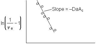
Figure 1. Dimensionless exit concentration function versus q
We have used data the concentration ratio, ( ψ e = CAe/CA0) at the exit, z=L, to evaluate the product DaAc. We will now evaluate the activity number, Ac, from the movement of the reaction front and the time it takes to break through at the end of the reactor, z=L.
H. Movement of the Reaction Front
Look at the exponential terms in Eqn (26) that are multiplied by DaAc. The arguments are zero when θ = ε and when \( \theta = \left( 1 + \frac{1}{A_c} \right) \varepsilon \). These relationships give the movement of two fronts. This front gives the dimensionless position of fresh gas interface
\( \varepsilon = \theta \)
\( z_1 = \frac{t}{\tau} L = \frac{t L}{L/U} = U t \)
This front gives the dimensionless position of the decay activity interface
\( \theta = \left( 1 + \frac{1}{A_c} \right) \varepsilon \)
Now that we have the product DaAc from the slope of Figure 1. At breakthrough of the activity front at the end of the reactor ε = 1
\( \frac{t_b}{\tau} = \theta_b = 1 + \frac{1}{A_c} \)
\( \theta_b - 1 = \frac{1}{A_c} \)
The breakthrough time is used to calculate the activity number
\( A_c = \frac{1}{\theta_b - 1} = \frac{\tau}{t_b - \tau} \)
I. Position of Reaction (Decay) Front
\( z_2 = \frac{A_c}{1 + A_c} U t \)
High Da
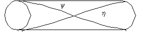
Low Da
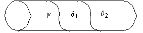
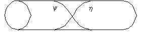
Figure 2. Profile of y and h
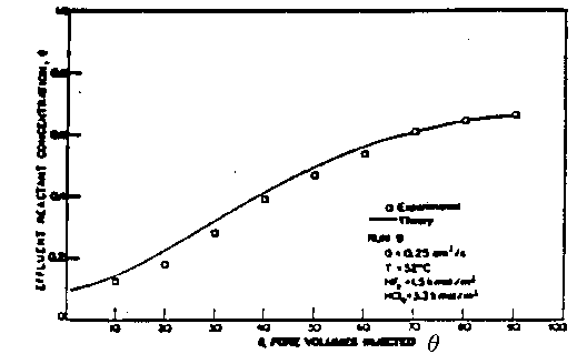
Figure 3. Comparison of Theory and Experiment
From Lund and Fogler Chem. Engrg. Sci. 31 p381 (1976).