Chapter 9: Reaction Mechanisms, Pathways, Bioreactions and Bioreactors
Topics
Active Intermediates / Free Radicals (PSSH)
TopAn active intermediate is a molecule that is in a highly energetic and reactive state It is short lived as it disappears virtually as fast as it is formed. They are short lived CA 10-14s and present in very low concentrations. That is, the net rate of reaction of an active intermediate, A*, is zero.
\( r_{A^*} = \sum r_{iA} = 0 \)
The assumption that the net rate of reaction is zero is called the Pseudo Steady State Hypothesis (PSSH)
The active intermediates reside in the trough of the reaction coordinate as shown below for \(\ce{C1-C2-C3-C4}\) Zewoil.
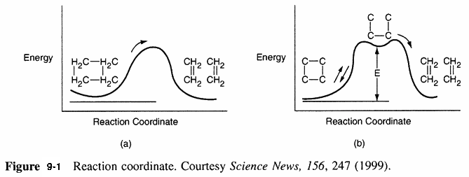
Hall of Fame Reaction
The reaction
\(\ce{2NO + O2 -> 2NO2}\)
has an elementary rate law
\( r_{NO_2} = k C_{NO}^2 C_{O_2} \)
However... Look what happens to the rate as the temperature is increased.
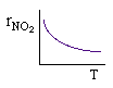
Why does the rate law decrease with increasing temperature?
Mechanism:
\(\ce{NO + O2 -> NO3^*} \quad (1)\)
\(\ce{NO3^* -> NO + O2} \quad (2)\)
\(\ce{NO3^* + NO -> 2NO2} \quad (3)\)
\( \frac{r_{NO_2}}{2} = r_{3NO_3^*} = -k_3 C_{NO_3^*} \cdot C_{NO} = k_3 [NO_3^*][NO] \)
Pseudo Steady State Hypothesis (PSSH)
The PSSH assumes that the net rate of species A* (in this case, NO3*) is zero.
\( r_{NO_3^*} \approx 0 = k_1 (NO)(O_2) - k_2 (NO_3^*) - k_3 (NO_3^*)(NO) \)
Solving for NO3*
\( NO_3^* = \frac{k_1 [NO][O_2]}{k_2 + k_3 [NO]} \)
\( r_{NO_2} = -2r_{3NO_3^*} = 2k_3 \frac{\left[ k_1 (NO)(O_2) \right] NO}{k_2 + k_3 (NO)} \)
\( r_{NO_2} = \frac{2 k_1 k_3 (NO)^2 (O_2)}{k_2 + k_3 (NO)} \)
\( k_2 \gg k_3 (NO) \)
\( r_{NO_2} = \frac{k_1 k_3}{k_2} (NO)^2 (O_2) = \frac{A_1 A_3}{A_2} e^{\frac{E_2 - (E_1 + E_3)}{RT}} (NO)^2 (O_2) \)
\( E_2 > (E_1 + E_3) \)
This result shows why the rate decreases as temperature increases.
Enzymes
TopMichaelis-Menten Kinetics
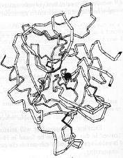
Enzymes are protein like substances with catalytic properties.
|
Enzyme unease. [From Biochemistry, 3/E by Stryer, copywrited 1988 by Lubert Stryer. Used with permission of W.H. Freeman and Company.] |
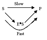
It provides a pathway for the substrate to proceed at a faster rate. The substrate, S, reacts to form a product P.
There are six classes of enzymes (\(E\)) and only six:
| 1. Oxidoreductases | \( AH_2 + B + E \rightarrow A + BH_2 + E \) |
| 2. Transferases | \( AB + C + E \rightarrow AC + B + E \) |
| 3. Hydrolases | \( AB + H_2O + E \rightarrow AH + BOH + E \) |
| 4. Isomerases | \( A + E \rightarrow \text{iso} - A + E \) |
| 5. Lyases | \( AB + E \rightarrow A + B + E \) |
| 6. Ligases | \( A + B + E \rightarrow AB + E \) |
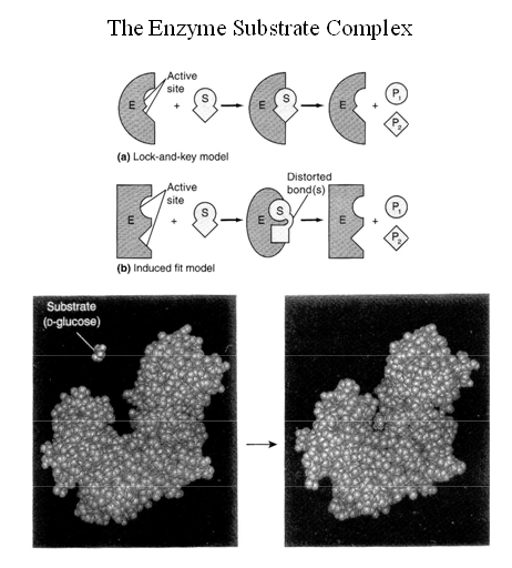
A given enzyme can only catalyze only one reaction. Urea is decomposed by the enzyme urease, as shown below.
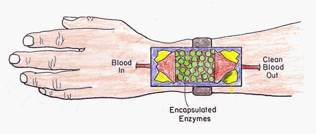
It has been proposed that an artificial kidney to remove urea from the blood could contain encapsulated enzymes and be worn externally.
\( \ce{NH2OCNH2 + UREASE -> 2NH3 + CO2 + UREASE} \)
\( \ce{S + E ->[H2O] P + E} \)
The corresponding mechanism is:
\( E + S \xrightleftharpoons[k_2]{k_1} E \cdot S \)
\( E \cdot S + W \xrightarrow{k_3} P + E \)
Michaelis-Menten Equation
\( r_p = -r_s = \frac{V_{max} S}{K_m + S} \)
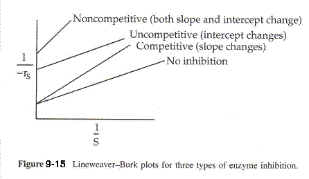
Inverting yields:
\( \frac{1}{-r_s} = \frac{1}{V_{max}} + \frac{K_m}{V_{max}} \left(\frac{1}{S}\right) \)
Types of Enzyme Inhibition
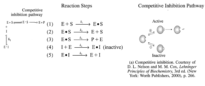
Reaction steps:
\( E + S \xrightarrow{k_1} E \cdot S \)
\( E \cdot S \xrightarrow{k_2} E + S \)
\( E \cdot S \xrightarrow{k_3} P + E \)
\( I + E \xrightarrow{k_4} E \cdot I \text{ (inactive)} \)
\( E \cdot I \xrightarrow{k_5} E + I \)
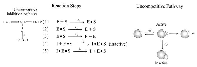
Reaction Steps:
\( E + S \xrightarrow{k_1} E \cdot S \)
\( E \cdot S \xrightarrow{k_2} E + S \)
\( E \cdot S \xrightarrow{k_3} P + E \)
\( I + E \cdot S \xrightarrow{k_4} I \cdot E \cdot S \text{ (inactive)} \)
\( I \cdot E \cdot S \xrightarrow{k_5} I + E \cdot S \)
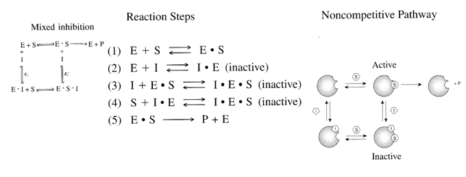
Reaction Steps:
\( E + S \rightleftharpoons E \cdot S \)
\( E + I \rightleftharpoons I \cdot E \text{ (inactive)} \)
\( I + E \cdot S \rightleftharpoons I \cdot E \cdot S \text{ (inactive)} \)
\( S + I \cdot E \rightleftharpoons I \cdot E \cdot S \text{ (inactive)} \)
\( E \cdot S \rightarrow P + E \)
Uncompetitive Substrate Inhibition
\( E + S \xrightleftharpoons[k_2]{k_1} E \cdot S \text{ (Inactive)} \)
\( S + E \cdot S \xrightleftharpoons[k_4]{k_3} S \cdot E \cdot S \text{ (Inactive)} \)
\( E \cdot S \xrightarrow{k_5} P + E \)
The Uncompetitive Substrate Inhibition rate law is
\( r_p = \frac{V_{max} S}{K_M + S \left( 1 + \frac{S}{K_I} \right)} = \frac{K_I V_{max} S}{S^2 + K_I S + K_M K_I} \)
Bioreactors
Top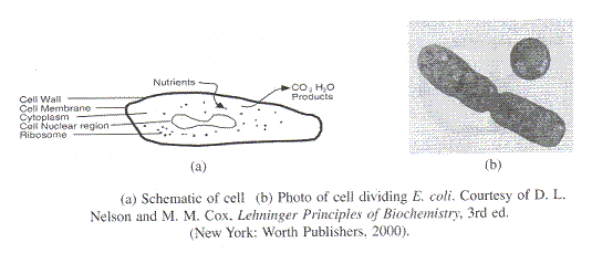
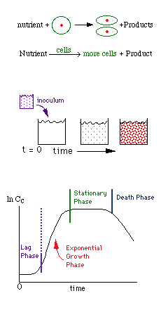
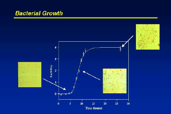
Data from Laboratory of H.S. Fogler taken by P.h.D Candidate Barry Wolf.
Rate Laws
\( r_2 = k_{\text{OBS}} \left| \frac{\mu_{\max} C_S}{K_S + C_S} \right| C_C \)
\( k_{\text{OBS}} = \left| 1 - \frac{C_P}{C_P^*} \right|^n \)
\( C_P^* \) = Where product concentration at which all metabolism ceases.
Stoichiometry
A. Yield Coefficients
\( Y_{c/s} = \frac{\text{mass of new cells formed}}{\text{mass of substrate consumed to produce new cells}}, \quad Y_{s/c} = \frac{1}{Y_{c/s}} \)
\( Y_{p/s} = \frac{\text{mass of product formed}}{\text{mass of substrate consumed to form product}} \)
B. Maintenance
\( m = \frac{\text{mass of substrate consumed for maintenance}}{\text{mass of cells} \cdot \text{time}} \)
\( -r_s = r_2 Y_{s/c} + r_d Y_{s/p} + m C_e \)
A word of caution on \( Y_{P/S} : \)
A. Growth Phase
\( -r_S = Y_{s/c} r_2 + m C_C \)
B. Stationary Phase
\( -r_{S_n} = m C_C + Y_{s_n/p} r_p \)
Mass Balances
Cell:
\( V \frac{dC_C}{dt} = v_0 C_{C_i} - v C_C + (r_2 - r_d) V \)
\( r_d = |k_n + k_{\text{ox}} C_{\text{tox}}^n| C_C \)
\( \Rightarrow \quad \text{Let } D = \frac{v_0}{V} \)
Also, \( C_{C_i} = 0 \), for most systems
Substrate:
\( V \frac{dC_S}{dt} = v_0 C_{S_i} - v C_S + r_2 V \)
\( C_S = C_{S0} \quad \text{at} \quad t = 0 \)
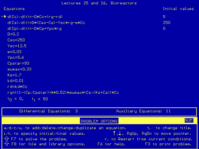
Polymath Setup
| 1.) |
d(Cc)/d(t) = - D*Cc + (rg - rd) |
| 2.) |
d(Cs)/d(t) = D*(Cso - Cs) - Ysc*rg - m*Cc |
| 3.) |
d(Cp)/d(t) = - D*Cp + Ypc*rg |
| 4.) |
rg = (((1 - (Cp/Cpstar))**0.52) * mumax*(Cs/(Ks + Cs))*Cc |
| 5.) |
D = 0.2 |
| 6.) |
kd = 0.01 |
| 7.) |
rd = kd*CC |
| 8.) |
Cso = 250 |
| 9.) |
Ypc = 5.6 |
| 10.) |
m = 0.3 |
| 11.) |
mumax = 0.33 |
| 12.) |
Ysc = 12.5 |
| 13.) |
Ks = 1.7 |
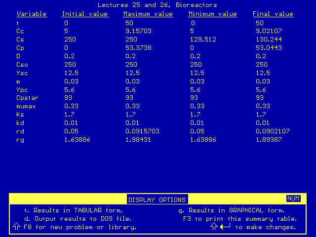
| Polymath Screen Shots |
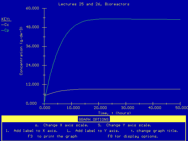
|
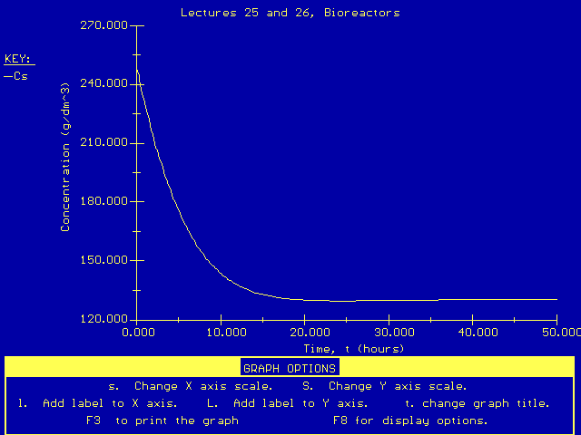
|
Wash Out:
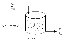
1. Neglect Death Rate and Cell Maintenance
2. Steady State
\( 0 = -u C_C + r_2 V \)
\( D C_C = r_2 = \frac{\mu_{\max} C_S}{K_S + C_S} C_C = \mu C_C \)
\( D = \mu = \frac{\mu_{\max} C_S}{K_S + C_S} \)
\( C_S = \frac{D K_S}{\mu_{\max} - D} \)
\( C_C = Y_{C/S} [C_{S0} - C_S] = Y_{C/S} \left[ C_{S0} - \frac{D K_S}{\mu_{\max} - D} \right] \)
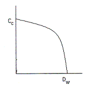
3. Washout
\( D_W = \frac{\mu_{\max} C_{S0}}{K_S + C_{S0}} \)
Maximum Production Rate
Production Rate = \( \dot{m}_c = v_o C_C \)
Dividing by the reactor volume, \( V \), which is constant
\( \frac{\dot{m}}{V} = D C_C \)
Substituting for \( C_C \)
\( D C_C = D Y_{C/S} \left( C_{S0} - \frac{D K_S}{\mu_{\max} - D} \right) \)
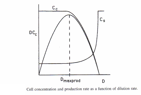
How does this figure relate to drinking a lot of fluids when you have an infection or cold?
Pharmacokinetics
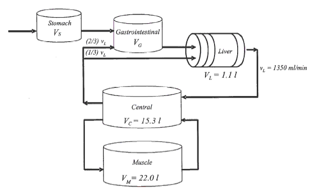
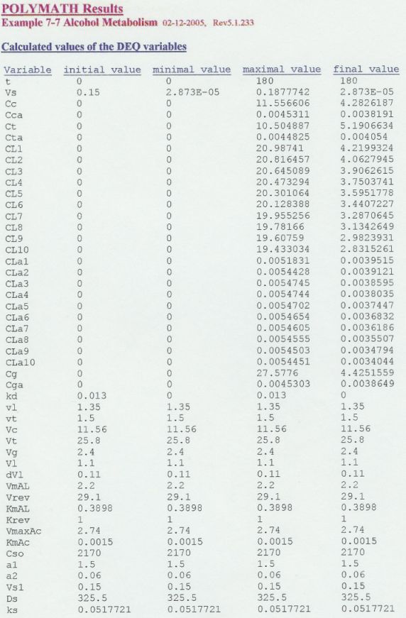
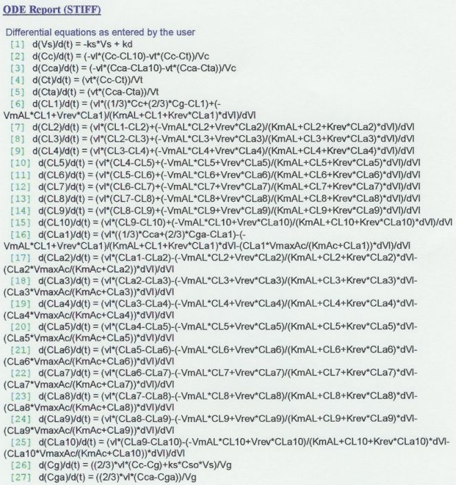
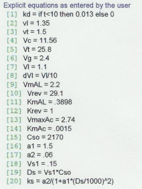
TopAlcohol Metabolism
\( \text{C}_2\text{H}_5\text{OH} \xrightleftharpoons{\text{ADH}} \text{CH}_3\text{CHO} + \text{H}_2\text{O} \xrightarrow{\text{ALDH}} \text{CH}_3\text{COOH} \)
\( \text{C}_2\text{H}_5\text{OH} + \text{NAD}^+ \xrightleftharpoons{\text{ADH}} \text{CH}_3\text{CHO} + \text{H}^+ + \text{NADH} \)
\[ - r_{ADC} = \frac{\left[V_{\max}^{\text{ADH}} C_{Ac} - V_{\text{rev}}^{\text{ADH}} C_{De}\right]}{K_{M}^{\text{ADH}} + C_{Ac} + K_{\text{rev}}^{\text{ADH}} C_{De}} \]
\( \text{NAD}^+ + \text{CH}_3\text{CHO} + \text{H}_2\text{O} \xrightarrow{\text{ALDH}} \text{CH}_3\text{COOH} + \text{NADH} + \text{H} \)
\[ - r_{De} = \frac{V_{\max}^{\text{ALDH}} C_{Ac}}{K_{M}^{\text{ALDH}} + C_{Ac}} \]
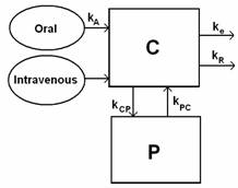
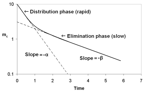
Drug Delivery
Polymerization
TopPolymers are macromolecules built up by the linking together of large numbers of much smaller molecules. The smaller molecules are called monomers and they repeat many times.
A polymer is a molecule made up of repeating structural (monomer) units.

Examples of Polymers

Poly (vinyl chloride)
Natural Polymers
Proteins
DNA/RNA
Cellulose
Fats
StarchSynthetic Polymers
Name Structural Repeating Unit (mer) Uses Poly (vinyl chloride) 
Pipes Polyethylene 
High density: Plastic cups
Low density: Sandwich bagsPolystyrene 
Coffee Cups Poly (acrylic acid) 
Superglue (Dow) Poly (cyano acrylate) 
Superglue Poly (vinyl acetate) 
Chewing gum Poly (vinyl alcohol) 
Shampoo/Thickener Poly (ethylene glycol) 
Stealth molecule Poly (methyl methacrylate) 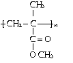
Plexiglas Poly (2-hydroxyethyl methacrylate) 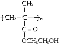
Contact Lenses Poly (tetra fluoro ethylene) 
Teflon Poly (ethylene terephthalate) 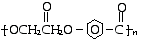
Coke bottles
Spinable fibers
A. Names/Nomenclature
Polymers that are synthesized from a single monomer are named by adding the prefix poly such as polyethylene. However, a parenthesis is placed after the prefix poly when the monomer has a substituted parent name or multiword name such as poly (acrylic acid) or poly (vinyl alcohol).
Homopolymers consist of a single repeating unit. All of the above are examples of homopolymers.
B. Polymer structure
1. Linear
Linear HDPE (70-90% crystalline)
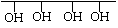
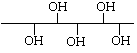
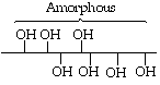
2. Stereoregularity Can Crystallize.
a.
Botactic = isotatic = same side
b.
Syndiotatic = alternating
c.
Atactic = random
Head to head (1,2 addition)

Head to tail (1,3 addition)
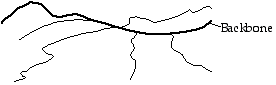
3. Branched Type A: Long Branches Off Backbone
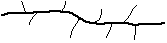
Branched Type B: Short Branches Off the Backbone
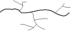
Branched Type C: Branches on Branches Off the Backbone
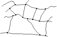
4. Cross linked
C. Copolymers
More than one repeating unit.
\( nA + nB \longrightarrow \{ A \}_n \{ B \}_n \)
For example, copolymers used to make records.
PVC - hard - irrigation pipes, hard to engrave
PVAc - easy to engrave
PVC + PVAc copolymer -> phonograph records (these are a thing of the past)
FIVE TYPES OF COPOLYMERS
Alternating
QSQSQS
Poly (vinyl acetate-alt-vinylchloride)
Block
QQQSSS
Poly (vinyl acetate-b-vinyl chloride)
Graph
QQQQQ
. . . . . |
. . . . . SSSSPoly (vinyl acetate-g-vinyl chloride
Random
QSSQQQSQSSS
Poly (VAc-co-VC)
Statistical
QSSQSQQSS
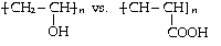
D. What affects polymer properties
• Chemistry
• Molecular Weight (\(\overline{MW}\)) and Molecular Weight Distribution
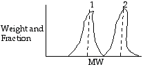

Weight Average Molecular Weight
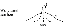

Molecular Weight Distribution
• Crystalinity
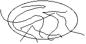
Amorphous Phase (Non-crystalline Phase) no order or orientation
|
|
Tg - characteristic of amorphous state Rubbery \( T_g \rightarrow \) glassy Below glass transition temperature, Tg, there is a cessation of virtually all molecular motion (vibration , rotation). |
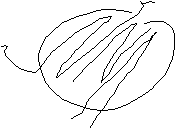
Crystalline Phase gives an order to the structure.
|
|
Order means crystallinity Crystalline \( T_m \rightarrow \) liquid Above the crystalline melting temperature, Tm, thre is no order. Fraction of total polymer that is in the crystalline state is the degree of crystallinity |
• Cross linking
• Branching
• Tacticity
• Head to head attachment vs. head to tail attachment
E. Molecular Weight (MW)
1. Measurement
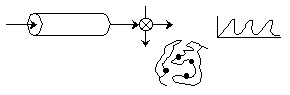
Membrane osmometry

Gel permeation chromatography
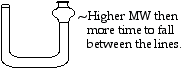
Viscosity
Light scattering
2. Calculation
Number average molecular weight \(\overline{M_n}\)
\(\overline{M_n} = \frac{\text{Total weight of polymer}}{\text{Number of moles present}} = \frac{W}{\sum N_i}\)
\(\overline{M_n} = \frac{\sum N_i M_i}{\sum N_i} = \sum y M_i\)
Weight average molecular weight \(\overline{M_w}\)
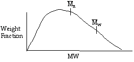
\(\overline{M_w} = \sum w_i M_i \quad \text{(Gives greater emphasis to larger molecules)}\)
\(w_i = \frac{N_i M_i}{\sum N_i M_i} = \frac{m_i}{W}\)
\(\overline{M_w} = \frac{\sum N_i M_i^2}{\sum N_i M_i}\)
Hence \(\overline{M_w}\) gives a truer picture of the average molecular weight.
\( 3H_2 + CO \xrightarrow{\text{Ni-Mo-Cu}} CH_4 + H_2O \)
3. Polydispersity
\( D = \frac{\overline{M_w}}{\overline{M_n}} \)
TWO TYPES OF HOMOGENEOUS POLYMERIZATION: STEP AND CHAIN
Step Polymerization. Monomer must be bifunctional. Polymerization proceeds by the reaction of two different functional groups. Monomer disappears rapidly, but molecular weight builds up slowly.
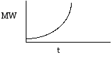
All species are treated as polymers. Mostly used to produce polyesters and polyamides.
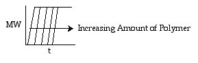
Chain Polymerization. Requires an initiator. Molecular weight builds up rapidly. Growing chains require 0.0001 to 1 to 10 seconds to terminate. Have high molecular weight polymers right at the start.
I. Step Polymerization
A. Functional Groups
\(-\text{OH}, -\text{COOH}, -\text{NH}_2, -\text{COCl}\)
1. Different functional groups on each end of monomer.
\(\text{H} \left[ \text{HN} - (\text{CH}_2)_5 - \text{CO} \right] \text{OH}\)
\(\text{A} \quad \quad \quad R_S \quad \quad \quad \quad \quad \text{B}\)
Structural Unit

Here the structural unit is the repeating unit.
2. Same functional groups on each end. Example: diamines and diols
Two structural units \( R_{s1} \) and \( R_{s2} \)
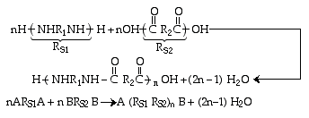
Repeating unit = \( R_{s1} R_{s2} = R_{R} \)
B. Polymerization Mechanism
Monomer dimer ----> trimer ----> tetrameter ----> Pentamer ---->
\( AR_1B + AR_1B \longrightarrow AR_2B + AB \)
\( AR_1B + AR_2B \longrightarrow AR_3B + AB \)
\( AR_2B + AR_3B \longrightarrow AR_5B + AB \)
\( AR_2B + AR_4B \longrightarrow AR_6B + AB \)
Monomer \( M \)
Dimer \( M + M \xrightarrow{k_1} M_2 \quad k_1 = 20 \times 10^{-4} \text{ dm}^3/\text{mol}\cdot s \)
Trimer \( M + M_2 \xrightarrow{k_2} M_3 \quad k_2 = 15 \times 10^{-4} \text{ dm}^3/\text{mol}\cdot s \)
Tetramer \( M_3 + M_1 \xrightarrow{k_3} M_4 \quad k_3 = 7.5 \times 10^{-4} \text{ dm}^3/\text{mol}\cdot s \)
Pentamer \( M_2 + M_2 \xrightarrow{k_4} M_4 \)
\( M_2 + M_3 \xrightarrow{k_5} M_5 \)
\( M_1 + M_4 \xrightarrow{k_5} M_5 \)
Hexamer \( M_1 + M_5 \xrightarrow{k_6} M_6 \)
\( M_2 + M_4 \xrightarrow{k_6} M_6 \)
\( M_3 + M_3 \xrightarrow{k_6} M_6 \)
For i > 2
\( k_i = 7.5 \text{ dm}^3/\text{mol}\cdot s \)
C. Structural Units
The number of structural units equals the number of bifunctional monomers present.
1. Monomers with different functional groups - one structural unit.
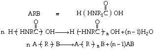
Here the repeating unit is the structural unit.
Let p = fraction of functional groups of either A or B that have reacted.
Let M = concentration of either A or B functional groups at time t.
Let M0 be the concentration of either A or B functional groups initially
\( M = M_0 - M_0 p = M_0 (1 - p) \)
Let N = total number (concentration) of polymer molecules present at time t.
Let N0 = total number of polymer molecules initially
Let MA = number of functional groups of A at time t.
Let MA0 = number of functional groups of A initially.
\( \overline{X}_n \) = number average degree of polymerization. It is the average number of structural units per chain.
\( \overline{X}_n = \frac{N_0}{N} \)
\( \overline{X}_n = \frac{M_0}{M} \)
therefore
\( \overline{X}_n = \frac{1}{1 - p} \)
\( \overline{M}_n \) the number average molecular weight.
\( \overline{M}_n = \overline{X}_n \overline{M}_s + M_{eg} \)
Where \(\overline{M}_s\) is the mean molecular weight of the structural units and \(M_{eg}\) is the molecular weight of the end group.
D. Monomers with Same End Group
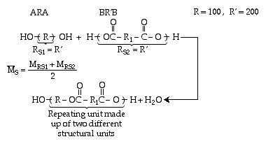
For a stoichiometric feed the number of A and B functional groups the same.

E. Stoichiometry Imbalance in the Feed
1. Stoichiometry Imbalance Type 1: Monomers with thesame end group and r not equal to 1
\( r = \frac{\text{number of A functional groups initially}}{\text{number of B functional groups initially}} = \frac{M_{A0}}{M_{B0}} \)
\( M_A = \text{number of A functional groups remaining} \)
\( M_B = \text{number of B functional groups remaining} \)
\( N = \text{Number of molecules remaining} = \frac{M_A + M_B}{2} \)
\( p = \text{fraction of A functional groups unreacted} \)
\( M_A = M_{A0}(1 - p) \)
\( M_B = M_{B0} - pM_{A0} = M_{B0} - pM_{B0} \frac{M_{A0}}{M_{B0}} = M_{B0} - p r M_{B0} = M_{B0} - p r M_{B0} = M_{B0}(1 - pr) \)
\( M_{A0} + M_{B0} = rM_{B0} + M_{B0} = (r + 1)M_{B0} \)
\( \overline{X}_n = \frac{M_{A0} + M_{B0}}{\frac{M_A + M_B}{2}} = \frac{M_{A0} + M_{B0}}{M_A + M_B} = \frac{(r + 1) M_{B0}}{M_{B0} [(1 - p) + 1 - rp]} \)
\( \overline{X}_n = \frac{r + 1}{1 + r - 2rp} \) / QED
The maximum number average chain length is greatly reduced if the initial feed is not exactly stoichiometric
If p = 1 then \( \overline{X}_n = \frac{r + 1}{1 - r} \)
2. Stoichiometry Imbalance Type 2: Monomers with different end groups. Monofunctional Monomer Present
\( A - R - A \quad . \quad B - R - B \quad . \quad B - C \)
\( r = \frac{\text{number of ARA molecules}}{\text{number of BRB molecules} + \text{number of BC molecules}} \)
\( [A - R - A]_o = [B - R - B]_o = M_{A0} \)
\( r = \frac{M_{A0}/2}{M_{A0}/2 + M_{B0}} = \frac{M_{A0}}{M_{A0} + 2M_{B0}} \)
\( [B - C]_o = M_{B0} \)
3. Stoichiometry Imbalance Type 3: Monomers with different end groups. Monofunctional Monomer Present
\( A - R - B + BC \)
\( r = \frac{N_{A0}}{N_{A0} + 2N_{B0}} \)
REACTION BETWEEN A DIOL (HOROH) AND A DIBASIC ACID (HOOCR1COOH)
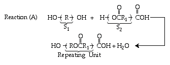
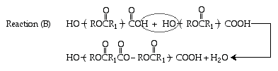

Let
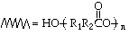
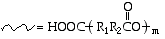
Then

Overall Reaction:
The Mechanism
Rate Law:
\( -r = k[H^+] (\sim OH)(-COOH) = -r_{\sim OH} \)
(1)

(2)

(3)

\( k_1 \cdot k_2 \cdot k_4 \gg \underline{k_3} \)
Let
-- =

~ =

The rate limiting step is Reaction (2)
\( -r = k_3 \left[ -\text{Q}^{+}(\text{OH})_2 \right] [\sim \text{OH}] \)
Assume Reaction (1) is essentially in equilibrium
\( \frac{\left[ -\text{C}(\text{OH})_2 (\text{A}^-) \right]}{\left[ \text{HA} \right] [\text{COOH}]} = K \)
\( r = k \left[ -\text{COOH} \right] \left[ \sim \text{OH} \right] \left[ \text{HA} \right] , \quad k = k_3 K \)
Case 1: The acid itself acts as a strong acid catalyst:
[HA] º [COOH] and Stoichiometric Feed.
\(-\frac{d[-\text{COOH}]}{dt} = k[-\text{COOH}]^2 [\sim \text{OH}] = k(-\text{COOH})^3\)
\(\frac{1}{(1 - p)^2} = 2kM_o^2 t + 1\)
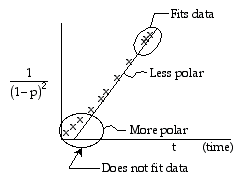
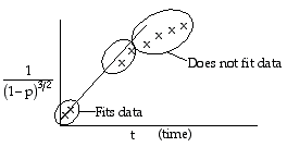
As the reaction proceeds and more ester is produced, the solution becomes less polar. As a result the uncatalyzed carboxylic acid becomes the major catalyst for the reaction, and the overall reaction order at high conversion is well described by a third order reaction (Case 1). The high conversion region is of primary importance because this region is where the high molecular weight polymers are formed.
At low conversions the solution is more polar and the proton, H+ is the more effective catalyst (Case 2) than the unionized carboxylic acid. Under these conditions, the reaction is self catalyzed and the reaction is 5/2 order.
Case 2: Self catalyzed but acid acts as a weak acid catalyst, not completely dissociated
[HA] = [-COOH]
\(\text{HA} \rightleftharpoons \text{H}^+ + \text{A}^- \quad , \quad \text{H}^+ = \text{A}^-\)
\(\text{H}^+ = \sqrt{K_A (\text{HA})}\)
\(-\frac{d[-\text{COOH}]}{dt} = k_3 K K_A^{1/2} [-\text{COOH}]^{3/2} [\sim \text{OH}] = k' [-\text{COOH}]^{5/2}\)
\(-\frac{dM}{dt} = k' M^{5/2}\)
\(\frac{1}{(1 - p)^{3/2}} = \frac{3}{2} k M_0^{3/2} t + 1\)
Case 3: External Acid Catalyzed H+ is constant
\(-\frac{d(-\text{COOH})}{dt} = k \left[ \frac{\text{H}^+}{k_1} \right] [-\text{COOH}][\sim \text{OH}]\)
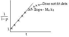
\(\frac{1}{1 - p} = M_0 k_1 t + 1\)
F. Kinetics of Step Polymerization
(1)
\(\text{ARB} + \text{ARB} \longrightarrow \text{AR}_2\text{B} + \text{AB}\)
\(\text{P}_1 + \text{P}_1 \xrightarrow{k} \text{P}_2 + \text{AB}\)
k is defined wrt the reactants
\(-r_{P_1} = 2k P_1^2\)
\(r_{P_2} = \frac{-r_{P_1}}{2} = k P_1^2\)
Why 2k? Because there are two ways A and B can react (thus, 2k)
\( A - R_n - B \)
\( A - R_m - B \)
(2)
\( P_1 + P_2 \longrightarrow P_3 \)
\( -r_{2P_1} = 2kP_1P_2 \)
(3)
\( P_1 + P_3 \longrightarrow P_4 \)
\( -r_{3P_1} = 2kP_1P_3 \)
\( r_{P_1} = r_{1P_1} + r_{2P_1} + r_{3P_1} \)
\( = -2kP_1^2 - 2kP_1P_2 - 2kP_1P_3 \)
For all reactions of P1
\( r_{P_1} = -2kP_1 \sum_{j=1}^{\infty} P_j = -2kP_1 M \), where \( M = \sum_{j=1}^{\infty} P_j \)
In general for j ? 2
\( r_{P_T} = r_j = k \sum_{i=1}^{j-1} P_i P_{j-i} - 2kP_j M \)
For j = 2
\( r_2 = k \sum_{i=1}^{1} P_i P_{j-1} - 2kP_2 M = kP_1^2 - 2kP_2 M \) \quad / QED
Mole balance on polymer of length j, in terms of the concentration Pj in a batch system
\( r_j = r_{P_j} = \frac{dP_j}{dt} \)
\( r_j = k \sum_{i=1}^{j-1} P_i P_{j-i} - 2kP_j M \)
\( \frac{dP_j}{dt} = k \sum_{i=1}^{j-1} P_i P_{j-i} - 2kP_j M \)
\( \frac{dM}{dt} = -kM^2 \) , \( \quad t = 0 \quad M = M_o \)
\( M = \frac{M_o}{1 + M_o k t} \)
\( P_1 = M_o \left( \frac{1}{1 + k M_o t} \right)^2 \)
\( P_2 = M_o \left( \frac{1}{1 + M_o k t} \right)^2 \left( \frac{M_o k t}{1 + M_o k t} \right) \)
If we proceed further it can be shown that
\( P_j = M_o \left( \frac{1}{1 + M_o k t} \right)^2 \left( \frac{M_o k t}{1 + M_o k t} \right)^{j-1} \)
\( P_j = M_o (1 - p)^2 (p)^{j-1} \)
\( p = \frac{M_o - M}{M_o} \)
Total number of polymer molecules (i.e. functional groups of either A or B) = \( \sum P_j = M \)
Mole fraction \( y_j = \frac{P_j}{M} = \frac{P_j}{M_o (1 - p)} \)
\( y_j = (1 - p) p^{j-1} \)
This is the Flory Distribution for the mole fraction of molecules with chain length j.
The weight fraction is just
\( P_j = M_o (1 - p)^2 p^{j-1} \)
\( w_{P_j} = (MW_s)_j M_o (1 - p)^2 p^{j-1} \)
W = total weight = \( MW_s M_o \)
\( w_j = \frac{w_{P_j}}{W} = \frac{w_{P_j}}{MW_s M_o} = j(1 - p)^2 p^{j-1} \)
G. Flory Distribution-Probability Approach
Rule: The probability of several events occurring successively in a particular way equals the product of the probabilities that each event happens that way.
P = probability that an A group will has reacted
(1-P) = probability group has not reacted.
A - R - B
HO - R C OO - H
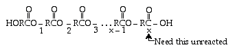
Probability of 1st link is P
Probability of 2nd link is P
Probability of A or B unreacted = (1 - P)
\( \text{Probability of Forming an } x\text{-mer} = \left( \text{Probability of } x-1 \text{ ester linkage} \right) \times \left( \text{Probability of unreacted } x\text{-group} \right) \)
\( = P^{x-1} (1-P) \)
\( M_x = M P^{x-1} (1-P) \)
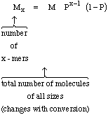
Mo = number of functional groups initially (no. of molecules)
M = number of functional groups remaining
\( p = \frac{M_O - M}{M_O} \)
\( M = M_O (1 - p) \)
\( M_x = M_O p^{x-1} (1 - p)^2 \Rightarrow \)
Number distribution function.
\( y_x = \frac{M_x}{M_O} = p^{x-1} (1 - p) \)
\( w_x = x M_{Ws} \cdot M_x \)
\( = M_O \left[ x (1 - p)^2 p^{x-1} \right] M_{Ws} \)
Weight distribution function
\( w_x = \frac{w_x}{M_O M_{Ws}} = x(1 - p)^2 p^{x-1} \)
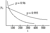
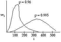
On a number average basis there will always be more monomer than polymer.
II. Chain Polymerization
A. Free Radical
Example: Polyethylene
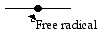
\( \text{I}-\text{CH}_2(\text{CH}_2)_n\text{CH}_2\bullet + \text{H}_2\text{C}=\text{CH}_2 \longrightarrow \text{I}-\text{CH}_2(\text{CH}_2)_{n+1}\text{CH}_2\bullet \)
Linear addition



Back biting
\(\Rightarrow\)
\(\Rightarrow\)
\(\text{HC}_2 = \text{CH}_2 +\)
\(\Rightarrow\)
\(\Rightarrow\)
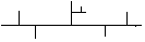
Branched Polyethylene resulting low density (0.92)
B. Cationic Polymerization
\(\text{BF}_3 + \text{H}_2\text{O} \longrightarrow \text{HOBF}_3^- + \text{H}^+\)
\[ \begin{array}{c} H^+ + & CH_2 = CH_2 \longrightarrow CH_3 - CH_2^+ \\ \end{array} \]
\[ \begin{array}{c} CH_3 - CH_2^+ + H_2C = CH_2 \longrightarrow CH_3CH_2 CH_2^+ , \text{etc.} \\ \end{array} \]
C. Anionic Polymerization
\(\text{A} \xrightleftharpoons{} \text{A}^- + \text{B}^+\)
\(\text{A}^- + \text{M} \longrightarrow R_1'\)
\(R_1' + \text{M} \longrightarrow R_2', \text{ etc.}\)
D. Ziegler-Natta Polymerization
Ziegler-Natta Catalyst \([\text{TiCl}_4\text{Al}(\text{CH}_2\text{CH}_3)_3]\)
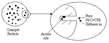
Steps in Polymer Chain Growth
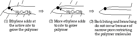
(4) Desorption from active site
\(\Rightarrow\)
+

to produce linear polymer: Eq. High Density Polyethylene (0.98) (HDPE)
Chain polymerizations require an initiator.
FREE RADICAL POLYMERIZATION
1. The Reaction
INITIATION
\(\text{I}_2 \xrightarrow{k_0} 2\text{I} \cdot \quad (\text{slow})\)
This reaction produces the formation of the Primary Radical
\(\text{I} \cdot + \text{M} \longrightarrow \text{R}_1 \cdot \quad (\text{fast})\)
PROPAGATION
\(\text{R}_1 \cdot + \text{M} \longrightarrow \text{R}_2 \cdot\)
\(\text{R}_{j-1} \cdot + \text{M} \longrightarrow \text{R}_j \cdot\)
TERMINATION
Transfer
Addition
To solvent
\(\text{R}_i \cdot + \text{S} \longrightarrow \text{P}_i + \text{S} \cdot\)
To monomer
\(\text{R}_i \cdot + \text{M} \longrightarrow \text{P}_i + \text{R}_1 \cdot\)
To chain transfer agent
\(\text{R}_i \cdot + \text{C} \longrightarrow \text{P}_i + \text{C} \cdot\)
To initiator
\(\text{R}_j \cdot + \text{I}_2 \longrightarrow \text{P}_j + \text{I} \cdot\)
\(\text{R}_j \cdot + \text{R}_k \cdot \longrightarrow \text{P}_{j+k}\)
Disproportionation
\(\text{R}_j \cdot + \text{R}_k \cdot \longrightarrow \text{P}_j + \text{P}_K\)
MORE ABOUT INITIATION
Types of initiators, homiletic, photo
\(\text{I}_2 \xrightarrow{k_o} 2\text{I}\)
\(\text{I} + \text{M} \xrightarrow{k_1} \text{R}_1\)
\(\left\{ \begin{array}{l} - r_{I_2} = k_o (\text{I}_2) \\ r_I = 2f k_o \text{I}_2 \end{array} \right.\)
\(r_i = r_{R_1} = k_i (\text{I}) (\text{M})\)
Typical Initiators for Homolytic Dissociation
\(\text{I}_2 \rightarrow 2\text{I}\)
Temperature Range
Initiator
(1)
50-70 \(^\circ \text{C}\)
Azobisisobutyranitride (ABIN)
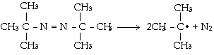
T 50° 70° 100° \( t_{1/2} \) 74 hr. 4.8 hr. 7.2 min.
(2)
70-90 \(^\circ \text{C}\)
Acetyl Peroxide

(3)
80-95 \(^\circ \text{C}\)
Benzyl Peroxide

Kinetics\(\frac{dI_2}{dt} = -k_o (I_2)\)
\(I_2 = I_{2o} e^{-k_o t}\)
\(\begin{array}{c} 10^{-2} \text{/s} < k_o < 10^{-6} \text{/s} \\ 25 \text{ kcal/mol} < E_a < 40 \text{ kcal/mol} \end{array}\)
Initiator Efficiency "f"f = fraction of radicals produced in the homolysis reaction that initiate polymer chains. It is a measure of waste of initiator.
How to determine f experimentally
- In AIBN measure N2 evolution compare number of radicals produced with number of polymer molecules obtained.
- Tag initiator 14C or 35S
- Use scavengers - to stop growth.
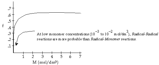
2. Free Radical Polymerization Kinetics
INITIATION
PSSH applied to initiator
(1) \( I_2 \rightarrow 2I \)
\( r_{1I} = 2f k_o (I_2) \)
(2) \( I + M \rightarrow R_1 \)
\( r_{2I} = -k_1 (I)(M) \)
\( r_{\text{1Net}} = 0 = 2f k_o (I_2) - k_1 (I)(M) \)
\( (I) = \frac{2f k_o I_2}{M k_1} \)
PROPAGATION
\( R_j + M \xrightarrow{k_P} R_{j+1} \)
\( -r_j = k_P M R_j \)
For all radicals the total rate of propagation
\( R_P = \sum (-r_j) = k_P M \sum R_j = k_P M R^* \)
\( R^* \) = total concentration of radicals (R1 + R2 + R3 . . . Rn)
Monomer balance
\( - r_m = r_1 + k_p M \sum R_j = k_i MI + k_p MR^* \)
Long Chain Approximation (LCA)
\( \frac{r_1}{R_p} \ll 1 \)
The rate of disappearance of monomer, -rm,
\( - r_m = k_p M R^* \)
\( \boxed{10^2 \text{ mol/dm}^3 \cdot s < k_p < 10^4 \text{ mol/dm}^3 \cdot s} \)
TERMINATION
1. Chain transfer
A.
To monomer
\( R_j + M \xrightarrow{k_M} P_j + R_1 \)
\( - r_{jm} = k_{tm} M R_j \)
Total rate of transfer for all radicals
\( r_{tm} = k_{tm} M R^* \)
B.
To solvent
\( R_j + S \xrightarrow{k_M} P_j + S \bullet \)
\( -r_{js} = k_{ts} M R_j \)
\( \boxed{r_{ts} = k_{ts} M R^*} \)
C.
Transfer to a chain transfer agent
\( R_j + C \xrightarrow{} P_j + C \bullet \)
\( -r_j = k_{tc} M P_j \)
\( \boxed{r_{tc} = k_{tc} M R^*} \)
D.
Transfer to initiator
\( R_j + I_2 \xrightarrow{} P_j + I \bullet \)
\( -r_{jI} = k_{tI} (I_2) R_j \)
\( \boxed{r_{tI} = k_{tI} (I_2) R^*} \)
2. Dispropriation Termination
\( R_j + R_k \xrightarrow{} P_j + P_k \)
\( -r_{tjk} = k_{td} R_j R_k \)
\( \boxed{-r_{tkj} = k_{td} R_j R_k} \)
Disproportionation
Define kd wrt reactants
\( R_1 + R_1 \xrightarrow{} P_1 + P_1 \)
\( r_{R_1} = k_d R_1^2 \)
i.e.
\( 2R_1 \xrightarrow{} 2P_1 \)
\( \frac{r_{R_2}}{2} = \frac{-r_{R_1}}{2} , \quad r_{P_1} = -r_{R_1} \)
\( R_1 + R_2 \xrightarrow{} P_1 + P_2 \)
\( R_1 + R_3 \xrightarrow{} P_1 + P_3 \)
\( R_2 + R_2 \xrightarrow{} P_2 + P_2 \)
\( R_2 + R_3 \xrightarrow{} P_2 + P_3 \)
\( r_{p_1,net} = r_{p_1,1} + r_{p_1,2} + r_{p_1,3} = k_d R_1^2 + k_d R_1 R_2 + k_d R_1 R_3 \)
\( = -k_d R_1 \sum R_j = k_d R_1 (R^*) \)
\( r_{p_2} = k_d R_1 R_2 + k_d R_2^2 + k_d R_2 R_3 + \dots \)
\( = k_d R_2 (R^*) \)
\( \sum r_{p_j} = k_d \sum R_j (R^*) = k_d (R^*)^2 \)
Net rate of termination of all radicals by dispropriation. For every dead polymer molecule that is formed, one live polymer radical is lost.
\( r_{tp} = \sum_{j=1}^{\infty} r_{pj} = -r_{td} = k_d (R^*)^2 = R_{td} \)
\( 10^6 \, \text{mol/dm}^3 \cdot s < k_d < 10^8 \, \text{mol/dm}^3 \cdot s \)
3. Addition Termination
\( R_j + R_k \longrightarrow P_{j+k} \quad \quad -r_{tjk} = k_a R_j R_k \)
where ka is defined wrt to the reactant.
The net rate of termination of j radicals will all the Rk radical (k = 1, 2, ?)
\( -r_{tj} = \sum_{k=1}^{n} -r_{tjk} \)
\( -r_{tj} = k_a R_j \left[ R_1 + R_2 + R_3 + \dots R_j + \dots \right] \)
\( = k_a R_j \sum R_j = k_a R_j R^* \)
The net rate of termination of all radicals is
\( R_t = \sum_{1}^{n} -r_{tj} = k_a \sum R_j R^* = k_a \left( R^* \right)^2 \)
PSSH Applied to All Free Radicals \( (R_{ta} = R_{ta}) \)
\( \sum r_j = r_1 - R_t = k_i (I) (M) - k_t (R^*)^2 = 0 \)
\( R^* = \sqrt{\frac{k_i (I) (M)}{k_t}} \)
Recall
\( k_i (I)(M) = 2k_o f(I_2) \)
\( R^* = \sqrt{\frac{2k_o f(I_2)}{k_t}} \)
Example Termination by the Initiator Primary Radicals, I
\( R_j + I \xrightarrow{k_u} P_j + I \)
\( r_t = k_t (R^*) (I) \)
\( r_p = k_p [M] R^* \)
\( r_i = k_i [M] (I) \)
\( r_t = r_i \)
\( R^* = \frac{k_i M}{k_t I} = \frac{k_i}{k_t I} \)
\( r_p = \frac{k_p k_i M^2}{k_t I} \)
Independent of Initiator Concentration
\( \ln \frac{M}{M_0} = \left( \frac{8 f k_p^2 I_{20}}{k_0 k_t} \right)^{1/2} \left[ \exp \left( \frac{-k_0 t}{2} \right) - 1 \right] \)
\( t \longrightarrow \infty \)
\( \ln \frac{M_0}{M_{\infty}} = \left( \frac{8 k_p^2 I_{20} f}{k_0 k_t} \right)^{1/2} \)
\( \ln \frac{1}{1 - p_{\infty}} = \left( \frac{8 k_p I_{20} f}{k_0 k_t} \right)^{1/2} \)
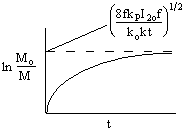
\( \ln (1 - p) = -\ln (1 - p_{\infty}) e^{\left[ \frac{-k_0}{2} - 1 \right]} \)
\( -\ln \left[ 1 - \frac{\ln (1 - p)}{\ln (1 - p_{\infty})} \right] = \frac{k_0}{2} t \)
Dead ended polymerization occurs when the initiator concentration decreases to such a low value, the half life of the polymer chains approximates half life of initiator
![Graph plotting -ln[1 - (ln(1 - p) / ln(1 - p∞))] against time (t) in hours. Two linear trends are shown, one labeled 80°C with a steeper slope and the other labeled 60°C with a gentler slope, indicating temperature-dependent reaction kinetics.](images/polymerization/image25.gif)
\( -\ln \left[ 1 - \frac{\ln(1 - p)}{\ln(1 - p_{\infty})} \right] \)
Polymerization of Isoprene initiated by azobisisolulyronitride.
Kinetic Chain Length
The kinetic chain length v is the average number of monomer molecules consumed (polymerized) per radial that initiates a polymer chain.
\( v = \frac{\text{rate of radical propagation}}{\text{rate of initiation}} \)
\( v = \frac{R_p}{R_i} = \frac{R_p}{R_t}, \quad (i.e. \ R_i = R_t) \)
\( \overline{X_n} = 2v \) termination by combination (addition)
\( \overline{X_n} = v \) termination by disproportionation
Chain Transfer
\( \overline{X_n} = \frac{R_p}{R_t + k_{tr,M} (R^*) [M] + k_{tr,S} [S] (R^*) + k_{tr,I} [I_2]} \)
\( R_p = k_p R^* M \)
In Principles of Polymerization 3/e by George Odian, the definition of Rt, the factor of 2 is incorrect but does not matter because it cancels out since Rt is dived by 2 in the denominator in later equations. Also note Eqn. (3-118a) in Odians is altogether incorrect.
Let the transfer coefficient be defined by
\( C_M = \frac{k_{tr,M}}{k_P}, \quad C_S = \frac{k_{tr,S}}{k_P}, \quad \text{and} \quad C_I = \frac{k_{tr,I}}{k_P} \)
\( \frac{1}{\overline{X_n}} = \frac{R_t}{R_p} + C_M + C_S \frac{S}{M} + C_I \frac{I_2}{M} \)
Term (1)
\( \frac{R_t}{R_p} = \frac{k_t (R^*)^2}{k_P R^* M} = \frac{k_t (k_P R^* M) R^*}{[k_P R^* M] k_P M} \)
Canceling terms
\( \frac{R_t}{R_p} = \frac{k_t R_p}{k_p^2 M^2} \)
Term (4)
\( \frac{I_2}{M} = \frac{?}{M} \)
\( (R^*)^2 = \frac{2 k_o I_{2f}}{k_t} \)
Solving for I2
\( I_2 = k_t \left( \frac{(R^*)^2}{2 k_o f} \right) \cdot \left( \frac{(M k_p)^2}{(M k_p)^2} \right) = \frac{k_t R_p^2}{2 f k_o k_p^2 M^2} \)
\( \frac{I_2}{M} = \frac{k_t R_p^2}{2 k_o f k_p^2 (M^3)} \)
The Mayo-Walling Equation
\( \frac{1}{\overline{X_n}} = \frac{k_t R_p}{k_p [M^2]} + C_M + C_S \frac{S}{M} + C_I \frac{k_t R_p^2}{2 k_p^2 k_o f [M^3]} \)
Let's neglect the term \( \left[ C_S \frac{S}{M} \right] \)
![Graph of 1/Xn versus Rp. The graph shows different slopes for different initiators and different CI values. The slope is represented by kt / (kp[M]^2). The intercept is labeled as CM.](images/polymerization/image39.gif)
For styrene
In benzyl peroxide
CM = 0.00006
CI = 0.055
In benzene
CS = 2.3 ´ 10?6
In Butyl mercaptan
CS = 21.1
Increasing the initiator concentration decreases \( \overline{X_n} \)
Increasing the monomer concentration increases \( \overline{X_n} \)
Further determination of Rate Constant
\( \frac{dM}{dt} = \alpha M I_2^{\frac{1}{2}} \)
1. Dilatometry
Volume charge
2. Spectroscopically measure I2(t) and M(t)
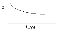
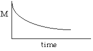
B. Batch - Method of Initial Rates
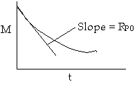
Many experiments
\( R_{P0} = \alpha I_{o}^{1/2} M_{o} \)
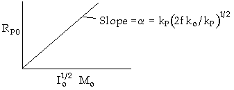
Steady State Measurement
CSTR
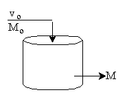
\( v_o M_o - v M + R_p V = 0 \)
\( v \approx v_o \)
\( R_p = \frac{v_o}{V} [M_o - M] \)
\( R_p = \alpha I_2^{\frac{1}{2}} M \)
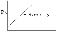
\( I_{\text{out}}^{\frac{1}{2}} M_{\text{out}} \)
No Chain Transfer
\( \overline{X_n} = \frac{k_p}{\left(2 f k_o k_t\right)^{1/2}} \frac{M_{\text{out}}}{I_{2\text{out}}^{1/2}} = \frac{\beta M_{\text{out}}}{\left(I_{2\text{out}}\right)^{1/2}} \)
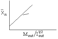
\( \alpha \times \beta = \frac{k_p}{k_t^{1/2}} \)
Determining Chain transfer Constants
A. Only transfer to chain transfer agent S
\( X_n = \frac{R_p}{R_t + R_s} \)
\( \frac{1}{X_n} = \frac{R_t}{R_p} + \frac{R_s}{R_p} \)
\( = \frac{k R^*}{k_p M} + \frac{k_{\text{tr},S} S}{k_p M} \)
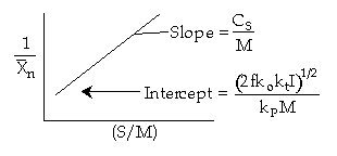
\( \frac{1}{X_n} = \frac{k_t R^*}{k_p M} + \frac{k_{\text{tr},S} S}{k_p M} = \frac{k_t}{k_p} \left[ \frac{2 k_o I_2}{k_t} \right]^{1/2} \frac{1}{M} + C_s \frac{S}{M} \)
Hold M and I constant, vary S
B. Transfer to monomer, initiation and a chain transfer agent
\( \frac{1}{X_n} = \frac{(2 f k_o k_t I_2)^{1/2}}{k_p M} + C_s \frac{S}{M} + C_I \frac{I_2}{M} + C_M \)
\( = \left[ \frac{(2 f k_o k_t I_2)^{1/2}}{k_p} + C_s S + C_I I_2 \right] \frac{1}{M} + C_M \)
Hold I and S constant, vary M
![Graph of 1/X̄ₙ versus 1/M with a straight-line trend. The slope is labeled as [ ] = S₁, and the intercept is labeled as Cₘ.](images/polymerization/image66.gif)
Change I and repeat, the intercept will be the same but slope will be different, S2. Change S and repeat S3. Three equations and 3 unknowns. Could also use regression.
Transfer Constants
A. To Monomer
0.00005 < CM < .0015
CM is generally small, however chain transfer to monomer for vinyl chloride is sufficiently high to limit the molecular weight so that the maximum molecular weight of PVC is 50,000 to 500,000.
B. To Initiator
CI is a function of both the initiator and the reaction
0.0008 < CI < 0.3
Peroxides are usually the strongest chain transfer agents.
C. To Chain Transfer Agent
\( \frac{1}{X_n} = \frac{k_p R_p}{k_p^2 [M]^2} + C_M + C_I \frac{k_p R_p^2}{k_p^2 f k_d [M]^3} + C_s \frac{S}{M} \)
\( \frac{1}{X_n} = \frac{1}{X_{no}} + C_s \frac{S}{M} \)
For styrene
0.000002 < CS < 21
(Benzene) < CS < (n Butyl mercaptan)
![Graph of (10⁵ / X̄ₙ) versus [S] / [M] with three labeled trend lines: C₂H₅φ, CH₃φ, and OH, increasing in slope.](images/polymerization/image68.gif)
Chain Transfer to Polymer, CP
Chain transfer to polymer produces branched polymers.
It is not important in determining CI, CM and CS because they are determined at low conversion.
CP involves the determination of the number of branches produced relative to the number of polymer molecules polymerized.
CP is the order of 10?4
The branching density, r , is the number of branches per monomer molecule polymerized.
\( \rho = C_p \left[ \frac{1}{p} \ln \frac{1}{1 - p} - 1 \right] \)
For CP = 10?4 and 80% conversion, there will be 1.0 branches per 104 monomer units polymerized. There is one branch for every 4,000 to 10,000 monomer units and for a polymer molecular weight of 105 ? 106 this corresponds to 1 polymer chain in 10 containing a branch.
Polyethylene
1. Short branches (less than 7 carbon atoms)
Formed by backbiting. Short branches out number the long branches by a fact of 20-50. They affect crystallinity giving maximum crystallinity of 60-70%.
2. Long branches ? formed by normal chain transfer to polymer.
Energetics (Free Radical)
\(\text{Initiation} \quad k_o = A_o e^{-\frac{E_o}{RT}} \quad 110 < E_o < 160 \quad \text{kJ/mol} \)
\(\text{Propagation} \quad k_p = A_p e^{-\frac{E_p}{RT}} \quad 15 < E_p < 40 \quad \text{kJ/mol} \)
\(\text{Termination} \quad k_t = A_t e^{-\frac{E_t}{RT}} \quad 2 < E_t < 20 \quad \text{kJ/mol} \)
\(\text{Transfer} \quad k_{tr} = A_{tr} e^{-\frac{E_{tr}}{RT}} \quad 40 < E_{tr} < 80 \quad \text{kJ/mol} \)
\( R_p \sim k_o^{1/2} k_p / k_t^{1/2} \)
\(\frac{d \ln (R_p)}{dT} \sim \left[ \frac{(2E_p + E_o) - E_t}{2RT^2} \right] \)
\( E_o > E_p > E_t \)
\(\frac{d \ln R_p}{dT} \text{ is } +, \quad \therefore R_p \uparrow \text{ as } T \uparrow \)
\(\bar{X}_n \sim k_p / (k_o k_t)^{1/2} \)
\(\frac{d \ln \bar{X}_n}{dT} = \left[ \frac{2E_p - (E_o + E_t)}{2RT^2} \right] \)
\(\therefore \bar{X}_n \downarrow \text{ as } T \uparrow \)
\(\frac{d \ln C}{dT} = \frac{E_{tr} - E_p}{RT^2}, \quad \text{normally } E_{tr} > E_p \)
Therefore chain transfer becomes more significant as temperature increases!!!
Chain Polymerization
Ionic Polymerization
Cationic

Used for monomers with electron releasing substituents
\( M_n A \rightleftharpoons M_n^+ A^- \rightleftharpoons M_n^+ \parallel A^- \rightleftharpoons M_n^+ + A^- \)
(a) (b) (c) (d)
e.g. alkoxy, 1,1?dealky
(a) covalent species, (b) tight ion pair, (c) loose ion pair, (d) free and highly solvated ion
Anionic

Used with monomers possessing electron withdrawing groups, e.g. nitride, carboxyl.
\( M_n A \rightleftharpoons M_n A^+ \rightleftharpoons M_n^- \parallel A^+ \rightleftharpoons M_n + A^+ \)
Anionic
High molecular weight. No chain-chain termination.
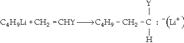
Initiation
Alkyllithium used because soluble in hydrocarbon solvents.
\( C_4H_9Li + CH_2 = CHY \rightarrow C_4H_9 - CH_2 - CYH \ :^- (Li^+) \)
Potassium amide
\( KNH_2 \xrightleftharpoons{K_e} H_2N:^− + K^+ \)
\( AB \xrightleftharpoons{} A^- + B^+ \)
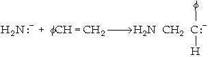
\( A^- + M \rightarrow R_1 \)
\( R_i = k_i [H_2N:^−][M] = \frac{k_i K [K_e H_2N][M]}{[K^+]} \)
Propagation
No effective termination - complete consumption of monomer to form living polymers.
\( H_2N = R_n^- + M \rightarrow H_2N - M_n M^- \)
\( R_n^- + M \rightarrow R_{n+1}^- \)
\( R_p = k_p [R_n^-][M] \)
Termination by:
a. Impurities
Moisture

\( R_{trH_2O} = k [R^-][H_2O] \)
b. Deliberate addition of chain transfer agent
c. Spontaneous
Hydride elimination, i.e.

Comparison with free radical polymerization
Free Radical: \( R_P = k_P [M][R^*] \)
Concentration of radicals is 10?9 to 10?7 mol/dm3
Anionic: \( R_P = k_P^{app} [M][M^-] \)
Concentration of propagation anions is 10?4 to 10?2 mol/dm3
In hydrocarbon solvents \( k_P^{\text{app}} \) is 10-100 times smaller than kP
In either solvents \( k_P^{\text{app}} \) is 10-100 times larger than kP
Benzene
Tetrahydrofuran
1,2-Dimethoxyethane
\( k_P^{\text{app}} \) 2
550
3,800
Other values are given in Odian p.412
Why do the rates of polymerization vary by several orders of magnitude in different solvents?
Kinetics of Ion/Ion Pair Initiation/Polymerization
Initiation
\( A^- (B^+) \rightleftharpoons A^- + B^+ \quad \text{ion/ion pair equilibrium} \)
\( A^- + M \xrightarrow{k_F} AM^- \quad \text{ion initiation} \)
\( AM_n^- + M \rightarrow AM_{n+1}^- \quad \text{ion propagation} \)
\( A^- (B^+) + M \xrightarrow{k_A^\pm} AM^- (B^+) \quad \text{ion pair initiation} \)
\( A^- (B^+) M_n^- + M \rightarrow A^- (B^+) M_{n+1}^- \quad \text{ion pair propagation} \)
Summing over all radicals
\( R_P = k_P^- [A^-][M] + k_P^\pm [A^- (B^+)][M] \)
where \( [A^-] \) is the concentration of \( [A^-] \) and all radicals initiated with \( [A^-] \) and \( \left[ A^- (B^+) \right] \) is the concentration of \( \left[ A^- (B^+) \right] \) and radicals initiated with \( \left[ A^- (B^+) \right] \)
We assume the ion and the ion pair are in equilibrium with the "salt."
\( K = \frac{\left[ A^- B^+ \right]}{\left[ A^- (B^+) \right]} \)
\( \left[ A^- \right] = \left[ B^+ \right] \)
\( \therefore \left[ A^- \right] = \left( K \left[ A^- (B^+) \right] \right)^{1/2} \)
Let \( [R^-] \) be the total concentration of all types of anionic living propagating centers.
\(\left[ R^- \right] = \left[ A^- \right] + \left[ A^- \left( B^+ \right) \right] = I_o\)
where Io is the total amount of initiator added.
\( I_o = \left[ A^- \right] + \left[ A^- \left( B^+ \right) \right] \)
\( \left[ A^- \left( B^+ \right) \right] = I_o - \left[ A^- \right] \)
\( R_p = k_p \left[ A^- \right] M + k_p^{\pm} \left[ I_o - \left[ A^- \right] \right] M \)
\( = k_p^{\pm} (I_o) M + \left( k_p^- - k_p^{\pm} \right) \left[ A^- \right] M \)
For small degrees of dissociation
\( \left[ A^- \left( B^+ \right) \right] \cong I_o \)
\( \left[ A^- \right] = \left[ K \left[ A^- \left( B^+ \right) \right] \right]^{1/2} = \left( K I_o \right)^{1/2} \)
\( R_p = \left( k_p^{\pm} I_o + \left( k_p^- - k_p^{\pm} \right) \left( I_o k \right)^{1/2} \right) M \)
\( R_p = k_{\text{app}} I_o M \)
\( R_p = k_{\text{app}} I_o M \)
\( k_{\text{app}} = k_p^{\pm} + \frac{\left( k_p^- - k_p^{\pm} \right) K}{I_o^{1/2}} \)
\( R^- = \sum R_j^- = I_o \)
![Graph of kapp (apparent rate constant) versus a variable on the x-axis with units (dm³/mol•s). The equation (1/T₀)^(1/2) = [R⁻T]^(1/2) is displayed below the graph.](images/polymerization/image102.gif)
\( k_p^- \approx 5 \times 10^4 \)
\( k_p^{\pm} \approx 80 \)
Differ by a factor of \( 10^3 \)
If \( K \sim 10^{28} \) and
\( \sqrt{K} \sim 10^{-4} \)
then
\( k_{\text{app}} = 80 + \frac{50,000 \times 10^{-4}}{I_o^{1/2}} \)
\( k_{\text{app}} = 80 + \frac{5}{I_o^{1/2}} \)
If \( K \sim 10^{26} \) then
\( k_{\text{app}} = 80 + \frac{50}{I_o^{1/2}} = 80 + \frac{50}{R^{-1/2}} \)
Polymerization of Styrene
\( \text{Li}^+ \)
\( \text{Na}^+ \)
\( \text{Cs}^+ \)
\( k_p^{\pm} \)
160
80
22
\( K \times 10^7 \)
2.2
1.5
0.02
\( k_p^- \times 10^{-4} \)
6.5
6.5
6.5
Data of Bhattacharya et al., J. Phys Chem. 69, p.612 (1965)
So we see that different solvents bring about different degrees of dissociation of the initiator resulting in different specific reaction rates.
Anionic Polymerization
1. Determining the living polymer concentration as a function of time
\(\text{AB} \rightleftharpoons \text{A}^- + \text{B}^+\)
For complete dissociation of the iniator
\(\text{A}^- + M \xrightarrow{k_o} R_1\)
\(R_1 + M \xrightarrow{k_p} R_2\)
\(R_j + M \xrightarrow{k_p} R_{j+1}\)
Assumptions
Initiation is instantaneous, R10 = Io
2. No termination
\(\text{I} + \text{M} \xrightarrow{k_o} R_1\)
\(R_1 + \text{M} \xrightarrow{k_p} R_2\)
\(R_{j-1} + \text{M} \xrightarrow{k_p} R_j\)
Case 1 ko >> kp Immediate rate formulation of primary radical
\( I = I_0 e^{-\frac{k_o}{k_p} \theta} \)
\(\frac{dR_1}{dt} = k_o M I - k_p M R_1\)
\( R_1 = \frac{I_0 k_o}{k_o - k_p} \left[ e^{-\theta} - e^{-\frac{k_o}{k_p} \theta} \right] \)
\(\frac{k_o}{k_p} \gg 1\)
\( I = I_0 e^{-\frac{k_o}{k_p} \theta} \)
\( R_1 = I_0 e^{-\theta} \)
\(\text{at } \theta = 0; \quad R_1 = R_{01} = I_0 \)
Propagation with No termination
\(\frac{dR_1}{dt} = -k_p [R_1][M]\)
\(\frac{dR_2}{dt} = k_p [R_1 - R_2][M]\)
\(\frac{dR_j}{dt} = k_p [R_{j-1} - R_j][M]\)
For the live polymer with the largest chain length n
\(\frac{dR_n}{dt} = k_p R_{n-1} M\)
Summing all these equations
\(\sum_{j=1}^{n} \frac{dR_j}{dt} = \frac{dR^-}{dt} = \sum R_j = 0\)
Constant live polymer concentration
\( R^- = R_{10} = I_0 \)
\(\text{Let } dq = k_p M \, dt\)
\(\frac{dR_1}{d\theta} = -R_1\)
\( t = 0, q = 0, R_1 = I_0 \quad R_1 = R_{10} e^{-\theta} \)
\(\frac{dR_2}{d\theta} = R_1 - R_2\)
\(\frac{dR_2}{d\theta} + R_2 = I_0 e^{-\theta}\)
\( R_2 = I_0 \theta e^{-\theta} \)
\( R_3 = I_0 \frac{\theta^2}{2 \times 1} e^{-\theta} \)
\( R_4 = I_0 \frac{\theta^3}{3 \times 2 \times 1} e^{-\theta} \)
\( R_j = I_0 \frac{\theta^{j-1}}{(j-1)} e^{-\theta} \)
\( y_j = \frac{\theta^{j-1}}{(j-1)} e^{-\theta} \)
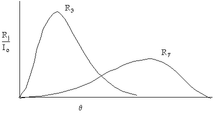
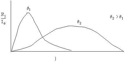
Convert back to real time from scaled time
\(\theta = \frac{M_0}{I_0} \left( 1 - e^{-I_0 k_p t} \right)\)
Very small \( t \) (i.e., small \( I_0 k_p t \))
\(\theta = M_0 k_p t\)
Very large \( t \) (i.e., large \( I_0 k_p t \))
\(\theta = \frac{M_0}{I_0}\)
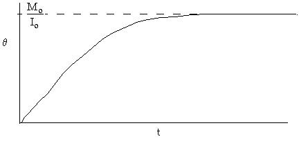
Distribution of molecular weights of living polymers
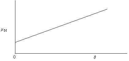
\(\text{NaCl} = \mu_N = (1 + \theta)\)
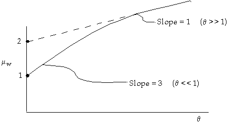
\(\mu_w = \frac{1 + 3\theta + \theta^2}{1 + \theta} = 1 + \theta + \frac{\theta}{1 + \theta}\)
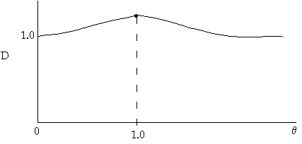
\(\text{D} = \frac{\mu_w}{\mu_n} = \frac{1 + 3\theta + \theta^2}{(1 + \theta)^2} = 1 + \frac{\theta}{(1 + \theta)^2}\)
Next consider a different set of initiation conditions
Case 2 ko = kp
\(\frac{dI}{dt} = -k_p I M\)
\(\frac{dI}{d\theta} = -I\)
\(I = I_o e^{-\theta}\)
\(R_1 = I_o \theta e^{-\theta}\)
\(R_2 = I_o \frac{\theta^2}{2!} e^{-\theta}\)
\(R_3 = I_o \frac{\theta^3}{3!} e^{-\theta}\)
\(R_n = \frac{I_o \theta^n}{n!} e^{-\theta}\)
Anionic Polymerization in a CSTR
\( I + M \xrightarrow{k_o} R_1 \)
\( R_1 + M \xrightarrow{k_p} R_2 \)
\( R_{j-1} + M \xrightarrow{k_p} R_j \)
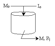
Monomer Balance
\(\tau \frac{dM}{dt} = M_0 - M - k_o (I) (M) \tau - k_p M \sum_{j}^{R^*} R_j \tau\)
Balance on \( R_1 \)
\(\tau \frac{dR_1}{dt} = R_{1f} - R_1 + \left( k_o (I) M - k_p R_1 M \right)\)
Balance on \( R_j \)
\(\tau \frac{dR_j}{dt} = 0 - R_j + k_p M \left[ R_{j-1} - R_j \right] \tau\)
Psuedosteady State Hypothesis (PSSH)
Case 1 ko is essentially (i.e., ko >> kp) infinite. Io is reacted immediately upon mixing with monomer to form R10
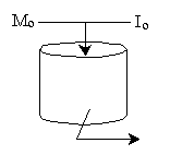
\(M_f, \quad R_{10} = R_{1f}\)
\(M_0 \gg I_0, \quad \therefore M_f = M_0\)
\(R_{10} = I_0 = \sum R_j = R^*\)
There is no initiator, \(I\), in the reactor
\(M = \frac{M_0}{1 + \tau k R^*} = \frac{M_0}{1 + \tau k_p R_{10}} = \frac{M_0}{1 + \tau k_p I_0}\)
\(R_j = \frac{R_{j-1} \tau k_p M}{1 + \tau k_p M}\)
\(R_j = \frac{R_{10}}{(1 + \tau k_p M)} \left( \frac{\tau k_p M}{1 + \tau k_p M} \right)^{j-1}\)
\(= R_{10} (1 - \phi) \phi^{j-1} = I_0 (1 - \phi) \phi^{j-1}\)
where \(\phi = \frac{\tau k_p M}{1 + \tau k_p M}\)
\(\mu_n = \frac{\sum j R_j}{\sum R_j} = \frac{\sum j R_j}{I_0}\)
\(\mu_n = \frac{1}{1 - \phi}\)
Substituting for \(M = \frac{M_0}{1 + \tau k_p I_0}\)
\(1 + \tau k_p M = 1 + \frac{\tau k_p M_0}{1 + \tau k_p I_0} = \frac{1 + \tau k_p (M_0 + I_0)}{1 + \tau k_p I_0}\)
\(\frac{\tau k_p M}{1 + \tau k_p M} = \frac{\tau k_p}{1/M + \tau k_p} = \frac{\tau k_p}{\frac{(1 + \tau k_p I_0)}{M_0} + \tau k_p}\)
\(R_j = R_{10} \frac{(1 + \tau k_p I_0)}{1 + \tau k_p (M_0 + I_0)} \left[ \frac{\tau k_p M_0}{1 + \tau k_p (I_0 + M_0)} \right]^{j-1}\)
Case 2 ko is finite
\(\tau \frac{dI}{dt} = I_0 - I - k_0 \tau M I\)
\(I = \frac{I_0}{1 + \tau k_0 M}\)
\(M = \frac{M_0}{1 + \tau k_0 (I) + \tau k_p I_0}\)
\(R_1 = \frac{\tau k_0 M I}{1 + \tau k_p M} \quad (R_{1f} = 0)\)
\(R_2 = \frac{R_1 k_p M \tau}{1 + \tau k_p M}\)
\(R_j = R_{j-1} \left( \frac{k_p M \tau}{1 + \tau k_p M} \right)\)
\(R_j = \frac{\tau k_0 M I}{1 + \tau k_p M} \left( \frac{\tau k_p M}{1 + \tau k_p M} \right)^{j-1}\)
\(R_j = \frac{\tau k_0 M I_0}{(1 + \tau k_p M)^{j} + \tau k_0 M} \left( \frac{\tau k_p M}{1 + \tau k_p M} \right)^{j-1}\)
\(j = 1\)
\(R_1 = \frac{\tau M I_0}{(1 + \tau k_p M) \left( \frac{1}{k_0} + \tau M \right)}\)
\(k_0 = \infty\)
\(R_1 = \frac{I_0}{1 + \tau k_p M}\)
* All chapter references are for the 1st Edition of the text Essentials of Chemical Reaction Engineering .