Chapter 9: Reaction Mechanisms, Pathways, Bioreactions and Bioreactors

Bifurcation Analysis

Substrate Inhibited Enzyme Reactions in a CSTR

Problem Statement

A substrate inhibiting enzyme reaction

$ S \xrightarrow{\text{Enzyme}} \text{products} $

is carried out in a CSTR with residence time t. The inlet concentration of the substrate is C_SO and the rate law is defined as

$-r_S = \frac{V_{\max} C_S}{K_m + C_S + K_I C_S^2} $ (1)

a) Reduce the material balance to show that

$ F(y) = y^3 - (y_o - 1)y^2 + (a + b - y_o)y - y_o a = 0 $ (2)

where

y = K_I C_S

y_o = K_I C_SO

a = K_m K_I

b = t V_max K_I

What is the maximum number of multiple steady states possible?

Solution Part (a)

b) Let A = y_o – 1 , B = a + b – y_o , C = y_o a

Show Eqn (2) can be put in the form

$ F(y) = y^3 - A y^2 + B y - C = 0 $ (3)

Solution Part (b)

c) Plot F(y) as a function of y (e.g. choose A=9, B=10, C=5.) Assuming the shape of the curve remains the same, sketch what happens as one varies A, B and C. Using the solution to (b), show the maximum and minimum points in F(y) occur at

$ y_{1,2} = \frac{A \pm \sqrt{A^2 - 3B}}{3} $ (4)

and that y₁ and y₂ are positive and real if

$ y_1 + y_2 > 0 $ (5)

$ y_1 y_2 > 0 $ (6)

Solution Part (c)

d) Discuss the fact that multiple steady states will occur if

$ F(y_1) F(y_2) \leq 0 $ (7)

Solution Part (d)

e) Show that multiple steady states can exist only if

(a + b) > y_o > 1 (8)

$ \left[ (K_M + \tau V_{\max}) > C_{S0} > \frac{1}{K_I} \right] $

and

27 C² – 18 ABC – A²B² + 4A³C + 4B³ < 0 (9)

Solution Part (e)

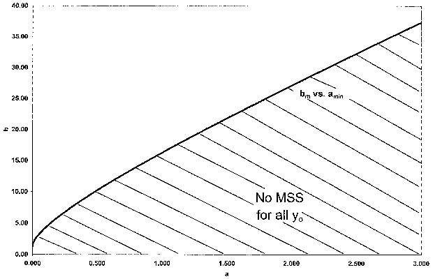
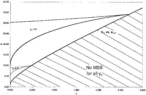
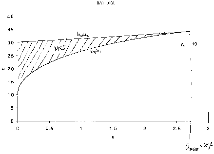
f) For y_o = 10, show the region of multiple steady states on a plot of “b” as a function of “a”. Hint: First use Polymath to find C and a function of B

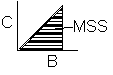Diagram featuring a right triangle with a hatched shading pattern, labeled with points B and C along the axes, and an annotation MSS extending from the hypotenuse. [Not to scale or shape]

What is the minimum value of “a” above which there will always be only one steady state? How will this minimum value of “a” change when y_o is changed?

Solution Part (f)

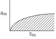
g) Develop a rough map to show

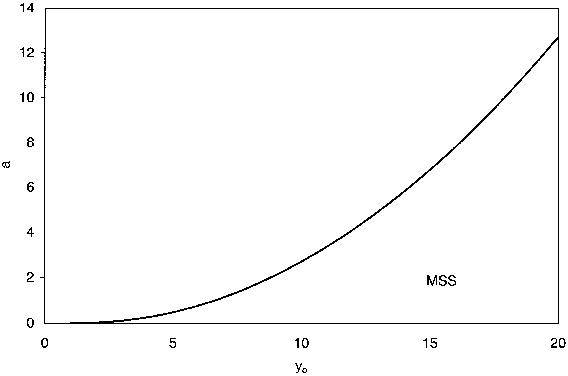
Graph with a shaded region under a curved line, bounded by the x-axis at bm and the y-axis at am. The shaded area represents a mathematical or physical concept.

Solution Part (g)

h) For very high substrate concentrations, what is the maximum number of multiple steady states possible? Show the region of MSS on a plot of b as a function of y_o.

Hint: For high C_S: $ -r_A = \frac{V_{\max} C_S}{K_I C_S^2} = \frac{V_{\max}}{K_I C_S} $

Solution:

Part a) CSTR Material Balance

$ v_o (C_{S0} - C_S) = V(-r_S) $

$ C_{S0} - C_S = \tau \frac{V_{\max} C_S}{K_m + C_S + K_I C_S^2} $

$ K_I C_{S0} - K_I C_S = \tau \frac{K_I V_{\max} C_S K_I}{K_m K_I + C_S K_I + K_I^2 C_S^2} $

$ y_o - y = \frac{b y}{a + y + y^2} $

where

$ y_o = K_I C_{S0} $

$ y = K_I C_S $

$ a = K_m K_I $

$ b = \tau K_I V_{\max} $

$ (y_o - y) \left( a + y + y^2 \right) = by $

$ a y_o + y_o y + y_o y^2 - a y - y^2 - y^3 = by $

$ y^3 - (y_o - 1) y^2 + (a + b - y_o) y - a y_o = 0 $

$ F(y) = y^3 - (y_o - 1) y^2 + (a + b - y_o) y - a y_o = 0 $

Because this is a cubic equation, three steady states are possible

Back to Part (b)

Part b)

$ A = y_o - 1 $

$ B = a + b - y_o $

$ C = y_o a $

$ F(y) = y^3 - (y_o - 1)y^2 + (a + b - y_o)y - a y_o = 0 $

$ F(y) = y^3 - A y^2 + B y + C = 0 $

Back to Part (c)

Part c)

@ y*

$\frac{dF}{dy} = 3y^2 - 2A y + B = 0$

$ y^*_ {1,2} = \frac{+ 2A \pm \sqrt{4A^2 - 4B3}}{2 \cdot 3} $

$ y^*_ {1,2} = \frac{A \pm \sqrt{A^2 - 3B}}{3} $

Back to Part (d)

Part d)

We need to find the condition when the above equation has three positive roots. Hence, graphically F(y) should be

$ \left[ F(\infty) \to \infty \quad \text{and} \quad F(-\infty) \to -\infty \right] $

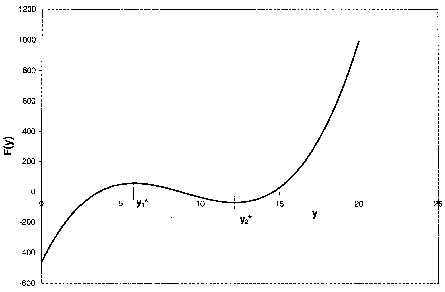
Graph of F(y) against y, showing a curve with a local maximum around y1* and a local minimum around y2*. The function increases sharply after y2*, with axis labels and markers indicating key points.

If F(y) is such that

Case I

$ F(y_1^*) F(y_2^*) \leq 0 $

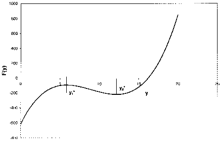
Graph of F(y) against y, showing a curve with a local maximum at y1* and a local minimum at y2*. The function decreases initially, peaks near y1*, dips slightly, and then rises steeply after y2*. Axis labels and markers indicate key points on the graph.

Case II

$ F(y_1^*) F(y_2^*) < 0 $

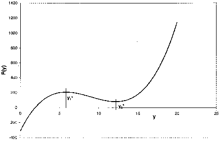
Graph of F(y) against y, showing a curve with a local maximum at y1* and a local minimum at y2*. The function initially increases, reaching a peak near y1*, then dips slightly before rising steeply after y2*. Axis labels and markers indicate key points on the graph.

Back to Part (e)

Part e)

Then there is only one real positive real root to F(y) = 0. Let’s assume that the points where

F'(y) = 0

are $ y_1^* $ and $ y_2^* $

For F(y) = 0 to have two positive real roots

$ y_1^* > 0 , y_2^* > 0 $ (1)

and

$ F(y_1^*) F(y_2^*) \leq 0 $ (2)

F'(y) = -3 y² - 2Ay + B = 0

$ y_{1,2}^* = \frac{A + \sqrt{A^2 - 3B}}{3} $

$ y_1^* + y_2^* = \frac{2A}{3} $

$ y_1^* y_2^* = \frac{B}{3} $

\text{For (1) i.e. } y_1^* > 0 \text{ and } y_2^* > 0

$ y_1^* + y_2^* = \frac{2A}{3} > 0 \Rightarrow A > 0 $

and

$ y_1^* y_2^* = \frac{B}{3} > 0 \Rightarrow B > 0 $

$ A > 0 \Rightarrow y_0 - 1 > 0 \Rightarrow y_0 > 1 $

$ B > 0 \Rightarrow a + b - y_0 > 0 \Rightarrow a + b > y_0 $

$\boxed{a + b > y_0 > 1} $ \quad (3)

For (2) i.e. $ F(y_1^*) F(y_2^*) \leq 0 $

$ \left[ y_1^{*3} - A y_1^{*2} + B y_1^* - C \right] \left[ y_2^{*3} - A y_2^{*2} + B y_2^* - C \right] \leq 0 $

$ \left[ (y_1^* y_2^*)^3 - A (y_1^* y_2^*)^2 (y_1^* + y_2^*) + B y_1^* y_2^* (y_1^{*2} + y_2^{*2}) \right. $

$ \left. - C (y_1^{*3} + y_2^{*3}) + A^2 (y_1^* y_2^*)^2 - AB (y_1^* y_2^*) (y_1^* + y_2^*) \right. $

$ \left. + AC (y_1^{*2} + y_2^{*2}) + B^2 (y_1^* y_2^*) - BC (y_1^* + y_2^*) + C^2 \right] \leq 0 $

Here,

\[ y_1^{*3} + y_2^{*3} = (y_1^* + y_2^*)^3 - 3 (y_1^* y_2^*) (y_1^* + y_2^*) \]

\[ y_1^{*2} + y_2^{*2} = (y_1^* + y_2^*)^2 - 2 (y_1^* y_2^*) \]

\[ (y_1^* + y_2^*) = \frac{2A}{3} \]

\[ (y_1^* y_2^*) = \frac{B}{3} \]

\[ \boxed{27C^2 - 18ABC - A^2B^2 + 4A^3C + 4B^3 \leq 0} \]

Using Maple

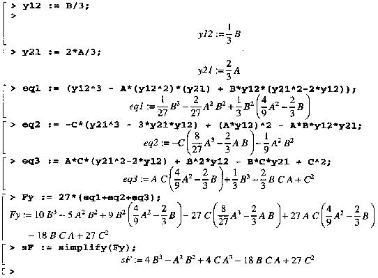
$Mathematical derivations showing symbolic equations involving variables A, B, and C. The expressions define y12 and y21, followed by three equations (eq1, eq2, and eq3) containing terms with exponents, products, and fractions. The final equation Fy combines the three expressions, followed by a simplified version sF.$

Hence (A) and (B) are the conditions for F(y) = 0 to have three positive real roots, i.e., three multiple steady states.

Back to Part (f)

For multiple steady states

$ 27C^2 - (18AB - 4A^3)C + (4B^3 - A^2B^2) \leq 0 $ (4)

$ C_1 = \frac{(18AB - 4A^3) + \sqrt{(18AB - 4A^3)^2 - 4 \times 27 \times (4B^3 - A^2B^2)}}{2 \times 27} $ (5)

$ C_2 = \frac{(18AB - 4A^3) - \sqrt{(18AB - 4A^3)^2 - 4 \times 27 \times (4B^3 - A^2B^2)}}{2 \times 27} $ (6)

For condition (1) to hold

C₁ ≤ C ≤ C₂

For y_o = 10

A = 9

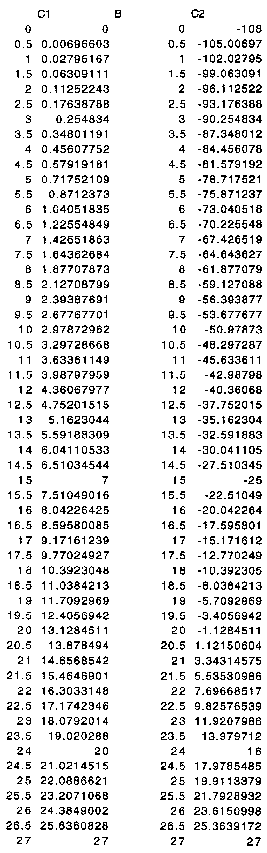
First compute C₁ and C₂ for various values of B as shown in Table 1

Mathematical equations defining differential equations and algebraic expressions. The equations involve parameters such as lambda (λ), initial values (yo), and constants (C1, C2). Expressions include square root terms, exponents, and algebraic manipulations related to variables A, B, and E. The final conditions are given as t0 = 0 and tf = 270.

Graph showing a C/B plot with a curved boundary and shaded region labeled MSS. The x-axis represents B, and the y-axis represents C. The graph includes functions labeled C1 - f1(B) and C2 - f2(B), marking upper and lower boundaries of the shaded region. The curve follows an increasing trend.

Table 1

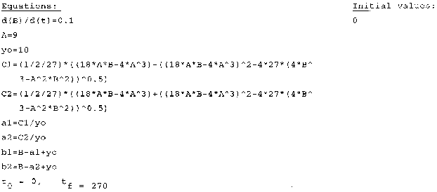
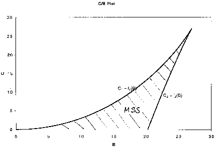
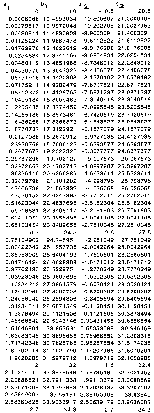
Table with three columns: C1, B, C2. C1 and B increase from 0 to 27, while C2 starts at -108 and rises to 27. Values are in decimal format and aligned in rows.

Coordinate Transformation

$ C = a y_0 $

$ B = a + b - y_0 $

Now

$ a_2 = \frac{C_2}{y_0} $

$ a_1 = \frac{C_1}{y_0} $

$ b_1 = B - a_1 + y_0 $

$ b_2 = B - a_2 + y_0 $

Plot $ a_2 $ as a function of $ b $ 2

Plot $ a_1 $ as a function of $ b $ 1

Table with five columns labeled a₁, b₁, a₂, b₂. Values in each column are decimal numbers increasing or decreasing systematically, with the last row showing rounded values.

Graph labeled b/a plot with b on the vertical axis and a on the horizontal axis. Two curves labeled b₂/a₂ and b₁/a₁ create a shaded region marked MSS. The upper curve approaches a constant value near 30. The lower curve increases rapidly before leveling off. Additional annotations include V₀ = 10 and Aₘₐₓ = 2.4 in the lower right corner.

Back to Part (g)

Part g)

Develop a plot of a versus y_o that divides the region into no MSS and MSS. Repeating the above procedure for various values of y_o, we will see that a_max increases as y_o increases.

$ F(C_S) = \frac{C_S}{\tau} - \frac{C_{S0}}{\tau} + \frac{V_m C_S}{K_m + C_S + K_I C_S^2} = 0 $

$ \frac{dF}{dC_S} = \frac{1}{\tau} + \frac{V_m (K_m + C_S + K_I C_S^2) - V_m C_S(1 + 2K_I C_S)}{(K_m + C_S + K_I C_S^2)^2} $

$ = \frac{1}{\tau} + \frac{V_m (K_m - K_I C_S^2)}{(K_m + C_S + K_I C_S^2)^2} = 0 $

$ F(C_S^*) = 0 \quad \Rightarrow \quad \frac{1}{\tau} = \frac{V_m C_S^*}{(C_{S0} - C_S^*)(K_m + C_S^* + K_I C_S^{*2})} $

$ F'(C_S^*) = 0 \quad \Rightarrow \quad \frac{1}{\tau} = \frac{V_m (K_I C_S^{*2} - K_m)}{(K_m + C_S^* + K_I C_S^{*2})^2} $

$ \Rightarrow \frac{C_S^*}{C_{S0} - C_S^*} = \frac{K_I C_S^{*2} - K_m}{K_m + C_S^* + K_I C_S^{*2}} $

$ \Rightarrow C_S^*(K_m + C_S^* + K_I C_S^{*2}) = (C_{S0} - C_S^*)(K_I C_S^{*2} - K_m) $

$ \Rightarrow K_m C_S^* + C_S^{*2} + K_I C_S^{*3} = K_I C_S^0 C_S^{*2} - K_m C_S0 - K_I C_S^{*3} + K_m C_S^* $

$ 2K_I C_S^{*3} + (1 - K_I C_{S0})C_S^{*2} + K_m C_{S0} = 0 $

$ y = K_I C_S $

$ y_o = K_I C_{S0} $

$ a = K_m K_I $

$ \Rightarrow \frac{2}{K_I^2} y^{*3} + (1 - y_o) \frac{y^{*2}}{K_I^2} + \frac{K_m C_{S0} K_I^2}{K_I^2} = 0 $

$ \Rightarrow 2y^{*3} + (1 - y_o) y^{*2} + a y_o = 0 $

$ \Rightarrow y^{*3} + \frac{(1 - y_o)}{2} y^{*2} + \frac{a y_o}{2} = 0 $

$ y^{*3} - A y^{*2} + B y - C = 0 $

$ \Rightarrow A = \frac{y_o - 1}{2}, \quad B = 0, \quad C = - \frac{a y_o}{2} $

For only one real root for y*

$ 27 C^2 + 4A^3 C \geq 0 \quad (\because C < 0) $

$ 27 C + 4A^3 \leq 0 $

$ \Rightarrow 27 C \leq 4A^3 $

$ \Rightarrow 27 \frac{-a y_o}{2} \leq 4 \frac{(y_o - 1)^3}{8} $

$ \Rightarrow a \geq + \frac{(y_o - 1)^3}{27 y_o} $

There will be no multiple steady states if $ \boxed{ a \geq \frac{(y_o - 1)^3}{27 y_o} } $

This is also mentioned in part (f) of the problem statement. $ \frac{(y_o - 1)^3}{27 y_o} $ is the minimum value of a above which there will always be only one steady state.

For y_o = 10 , a_min = $ \frac{(y_o - 1)^3}{27 y_o} = 2.7 $

(see b/a plot)

Multiple steady states may occur if

$ \boxed{a < \frac{(y_o - 1)^3}{27 y_o}} $

depending on the value of b (= t K_I)

Graph with variable a on the vertical axis and y₀ on the horizontal axis. The curve starts at the origin and rises steeply in a quadratic fashion. A region labeled MSS is marked in the lower right section of the graph.

At b_min

$ C_1 = C_2 = \frac{9AB - 2A^3}{27} $

$ a_{\min} y_o = \frac{9(y_o - 1)(b_m + a_m - y_o) - 2(y_o - 1)}{27} $

$ 9(y_o - 1)(b_m + a_m - y_o) = 27 a_m y_o + 2(y_o - 1)^3 $

$ b_m = (y_o - a_m) + \frac{[27 a_m y_o + 2(y_o - 1)^3]}{9(y_o - 1)} $

$ b_m = \left( y_o - \frac{(y_o - 1)^3}{27 y_o} \right) + \left[ \frac{(y_o - 1)^3 + 2(y_o - 1)^3}{9(y_o - 1)} \right] $

$ = \left[ y_o - \frac{(y_o - 1)^3}{27 y_o} + \frac{1}{3} (y_o - 1)^2 \right] $

$ = \left[ y_o + \frac{(y_o - 1)^2}{3} \left( 1 - \frac{y_o - 1}{9 y_o} \right) \right] $

$ \boxed{b_m = y_o + \frac{(y_o - 1)^2}{27 y_o} (8 y_o + 1)} $

Graph showing the relationship between variable a on the horizontal axis and variable b on the vertical axis. A curved boundary separates the graph into two regions, with the lower region shaded and labeled 'No MSS for all y₀'. The boundary is labeled 'bₘ vs. aₘᵢₙ'.

Graph showing the relationship between variable a on the horizontal axis and variable b on the vertical axis. The plot includes curves labeled y₀ = 5 and y₀ = 10. A curved boundary labeled 'bₘ vs. aₘᵢₙ' separates the graph into two regions, with the lower region shaded and labeled 'No MSS for all y₀'.

Back to Part (h)

Back to Chapter 9