Chapter 5: Isothermal Reactor Design: Conversion
Topics
- Algorithm for Isothermal Reactor Design
- Applications/Examples of CRE Algorithm
- Reversible Reactions
- ODE (Polymath) Solutions to CRE Problems
- General Guidelines for California Problems
- PBR with Pressure Drop
- Engineering Analysis
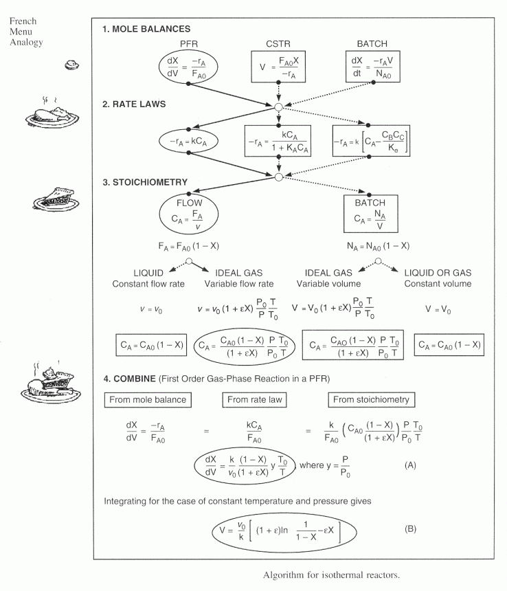
Algorithm for Isothermal Reactor Design
TopFor the $5^{th}$ edition $\frac{P}{P_o}$ equals $p$ i.e. $p = \frac{P}{P_o}$. In the $4^{th}$ and earlier editions $y = \frac{P}{P_o}$
- Mole Balance and Design Equation
- Rate Law
- Stoichiometry
- Combine
- Evaluate
- Graphically (Chapter 2 plots)
- Numerical (Quadrature Formulas Chapter 2 and appendices)
- Analytical (Integral Tables in Appendix)
- Software Packages (Appendix - Polymath)
Example: The elementary liquid phase reaction
\(2A \rightarrow B\)
is carried out isothermally in a CSTR. Pure A enters at a volumetric flow rate of 25 dm3/s and at a concentration of 0.2 mol/dm3.
What CSTR volume is necessary to achieve a 90% conversion when k = 10 dm3/(mol*s)?
Mole Balance
\(V = \frac{F_{A0}X}{-r_A}\)
Rate Law
\(-r_A = kC_A^2\)
Stoichiometry
liquid phase (v = vo)
\(F_{A0} = v_0C_{A0}\)
\(F_A = vC_A = v_0C_A\)
\(C_A = \frac{F_A}{v} = \frac{F_A}{v_0} = \frac{F_{A0}(1 - X)}{v_0}\)
\(C_A = C_{A0}(1 - X)\)
Combine
\(V = \frac{v_0 C_{A0} X}{kC_{A0}^2 (1 - X)^2} = \frac{v_0 X}{kC_{A0} (1 - X)^2}\)
Evaluate
at X = 0.9,
\(V = \frac{25 \, \mathrm{dm^3/s} \cdot (0.90)}{\left(10 \, \mathrm{dm^3/(mol \cdot s)}\right) \cdot \left(0.2 \, \mathrm{mol/dm^3}\right) \cdot (1 - 0.9)^2}\)
V = 1125 dm3
Space Time
\(\tau = \frac{V}{v_o} = \frac{1125 \, \mathrm{dm^3}}{25 \, \mathrm{dm^3/s}} = 45 \, \mathrm{s}\)
Here are some links to example problems. You could also use these problems as self tests.
Videos
The following humorous videos were made by Professor Lane's 2008 Chemical Reaction Engineering class at the University of Alabama, Tuscaloosa.
Applications/Examples of the CRE Algorithm
TopGas Phase Elementary Reaction
2A → B
Additional Information:
- Only A is fed
- P0 = 8.2 atm
- T0 = 500 K
- CA0 = 0.2 mol/dm3
- k = 0.5 dm3/mol-s
- vo = 2.5 dm3/s
Solve for X = 0.9
Applying the algorithm to the above reaction occurring in a Batch,
CSTR, and PFR.
| Batch | CSTR | PFR |
|---|---|---|
|
Mole Balance: \( t = N_{A0} \int_{0}^{X} \frac{dX}{-r_A} \) |
Mole Balance: \( V = \frac{F_{A0} X}{-r_A} \) |
Mole Balance: \( t = F_{A0} \int_{0}^{X} \frac{dX}{-r_A} \) |
|
Rate Law: \( -r_A = kC_A^2 \) Gas: \( V = V_0 \) (e.g., constant volume steel container) |
Rate Law: \( -r_A = kC_A^2 \) Gas: \( T = T_0, P = P_0 \) |
Rate Law: \( -r_A = kC_A^2 \) Gas: \( T = T_0, P = P_0 \) |
|
Stoichiometry: \( C_A = \frac{N_A}{V} = \frac{N_{A0}(1 - X)}{V_0} \) \( C_A = C_{A0}(1 - X) \) \( C_B = \frac{N_B}{V} = \frac{N_{A0} \left( + \frac{1}{2} X \right)}{V_0} \) \( C_B = \frac{C_{A0} X}{2} \) |
Stoichiometry: \(\text{Per Mole of A:}\) \(\text{A} \rightarrow \frac{\text{B}}{2}\) \(\varepsilon = 1.0 \left( \frac{1}{2} - 1 \right) = -0.5\) \(C_A = \frac{F_A}{\nu} = \frac{F_{A0}(1 - X)}{\nu_0(1 + \varepsilon X)}\) \(C_A = C_{A0} \frac{(1 - X)}{(1 + \varepsilon X)}\) \(C_B = \frac{F_B}{\nu} = \frac{F_{A0}\left(\frac{1}{2}X\right)}{\nu_0(1 + \varepsilon X)}\) \(C_B = \frac{C_{A0}X}{2(1 + \varepsilon X)}\) |
Stoichiometry: \(\text{Per Mole of A:}\) \(\text{A} \rightarrow \frac{\text{B}}{2}\) \(\varepsilon = 1.0 \left( \frac{1}{2} - 1 \right) = -0.5\) \(C_A = \frac{F_A}{\nu} = \frac{F_{A0}(1 - X)}{\nu_0(1 + \varepsilon X)}\) \(C_A = C_{A0} \frac{(1 - X)}{(1 + \varepsilon X)}\) \(C_B = \frac{F_B}{\nu} = \frac{F_{A0}\left(\frac{1}{2}X\right)}{\nu_0(1 + \varepsilon X)}\) \(C_B = \frac{C_{A0}X}{2(1 + \varepsilon X)}\) |
|
Combine: \(t = \frac{1}{kC_{A0}} \int_{0}^{X} \left[\frac{1}{(1 - X)^2}\right] dX\) |
Combine: \(V = \frac{F_{A0} X (1 - 0.5X)^2}{kC_{A0}^2 (1 - X)^2}\) |
Combine: \(V = \frac{F_{A0}}{kC_{A0}^2} \int_{0}^{X} \frac{(1 - 0.5X)^2}{(1 - X)^2} \, dX\) |
|
Integrate: \(t = \frac{1}{kC_{A0}} \left[ \frac{X}{1 - X} \right]\) |
Integrate: |
Integrate: \( V = \frac{F_{A0}}{kC_{A0}^2} \left( 2\epsilon(1+\epsilon)\ln(1-X) + \epsilon^2X + \frac{(1+\epsilon)^2X}{1-X} \right) \) |
|
Evaluate: \[ kC_{A0} = \left( 0.2 \, \frac{\text{dm}^3}{\text{mol} \cdot \text{s}} \right) \left( 0.5 \, \frac{\text{mol}}{\text{dm}^3} \right) = 0.1 \, \text{s}^{-1} \] \[ kC_{A0} = 0.1 \, \text{sec}^{-1} \] |
Evaluate: \[ kC_{A0}^2 = 0.5 \, \frac{\text{dm}^3}{\text{mol} \cdot \text{s}} \left( 0.2 \, \frac{\text{mol}}{\text{dm}^3} \right)^2 = 0.02 \, \frac{\text{mol}}{\text{dm}^3 \cdot \text{s}} \] \[ V = \frac{0.5 \, \frac{\text{mol}}{\text{s}} (0.9) \left(1 - 0.5(0.9)\right)^2}{0.02 \, \frac{\text{mol}}{\text{dm}^3 \cdot \text{s}} \left(1 - 0.9\right)^2} \] |
Evaluate: \[ F_{A0} = 0.5 \, \frac{\text{mol}}{\text{s}} \] \[ kC_{A0}^2 = 0.02 \, \frac{\text{mol}}{\text{dm}^3 \cdot \text{s}} \] \[ V = \frac{0.5 \, \frac{\text{mol}}{\text{s}} (0.9)}{0.02 \, \frac{\text{mol}}{\text{dm}^3 \cdot \text{s}}} \left( 2(-5)(1-5)\ln(1-0.9) + (-5)^2(0.9) + \frac{(1-5)^2(0.9)}{1-0.9} \right) \] |
|
For X = 0.9: \[ t = \left( \frac{1}{0.1 \, \text{s}^{-1}} \right) \left( \frac{0.9}{1-0.9} \right) \] \[ t = 90 \, \text{sec} \] |
For X = 0.9: \( V = 680.6 \, \text{dm}^3 \) \( \tau = \frac{V}{v_0} = 272.3 \, \text{s} \) |
For X = 0.9: \( V = 90.7 \, \text{dm}^3 \) \( \tau = \frac{V}{v_0} = 36.3 \, \text{s} \) |
Reversible Reactions
TopTo determine the conversion or reactor volume for reversible reactions, one must first calculate the maximum conversion that can be achieved at the isothermal reaction temperature, which is the equilibrium conversion. (See Example 3-8 in the text for additional coverage of equilibrium conversion in isothermal reactor design.)
Equilibrium Conversion, Xe
From Appendix C:
\( K_C = \frac{C_C^c C_D^d}{C_A^a C_B^b} \)
Example: Determine Xe for a PFR with no pressure drop, P = P0
Given that the system is gas phase and isothermal, determine the reactor volume when X = 0.8 Xe.
Reaction Additional Information
2A ⇌ B
- CA0 = 0.2 mol/dm3
- k = 2 dm3/mol-min
- KC = 100 dm3/mol
- FA0 = 5 mol/min
First calculate Xe:
\(K_C = \frac{X_e (1 + \epsilon X_e)}{2C_{A0} (1 - X_e)^2}\)
Xe = 0.89
X = 0.8Xe = 0.711
ODE (Polymath) Solutions to CRE Problems
Top| Algorithm Steps | Polymath Equations |
|---|---|
| Mole Balance | \( \frac{dX}{dV} = -\frac{r_A}{F_{A0}} \) |
| Rate Law | \( r_A = -k \left( (C_A)^2 - \frac{C_B}{K_C} \right) \) |
| Stoichiometry |
\( C_A = \frac{C_{A0} (1 - X)}{1 + \epsilon X} \) \( C_B = \frac{C_{A0} X}{2 (1 + \epsilon X)} \) |
| Parameter Evaluation |
\( \epsilon = -0.5 \), \( C_{A0} = 0.2 \, \text{mol/dm}^3 \), \( k = 2 \) \( F_{A0} = 5 \), \( K_C = 100 \) |
| Initial and Final Values | \( X_0 = 0 \), \( V_0 = 0 \), \( V_f = 500 \) |
Polymath Screen Shots
Equations
Plot of X vs. V
Results in Tabular Form
A volume of 94 dm3 (rounding up from slightly more than 93 dm3) appears to be our answer.
\( V = 94 \, \text{dm}^3 \)
General Guidelines for California Problems
TopEvery state has an examination engineers must pass to become a registered professional engineer. In the past there have typically been six problems in a three hour segment of the California Professional Engineers Exam. Consequently one should be able to work each problem in 30 minutes or less. Many of these problems involve an intermediate calculation to determine the final answer.
Some Hints:
|
PBR with Pressure Drop
TopNote: Pressure drop does NOT affect liquid phase reactions
Sample Question:
Analyze the following second order gas phase reaction that occurs isothermally in a PBR:
\( A \rightarrow B \)
Mole Balance
\( F_{A0} \frac{dX}{dW} = -r'_A \)
Must use the differential form of the mole balance to separate variables
Rate Law
Second order in A and irreversible:
\(-r'_A = kC_A^2\)
Stoichiometry
\(C_A = \frac{F_A}{\nu} = C_{A0} \frac{(1-X)}{(1+\epsilon X)} \frac{P \, T_0}{P_0 \, T}\)
Isothermal, T = T0
\(C_A = C_{A0} \frac{(1-X)}{(1+\epsilon X)} \frac{P}{P_0}\)
Combine
\(\frac{dX}{dW} = \frac{kC_{A0}^2}{F_{A0}} \frac{(1-X)^2}{(1+\epsilon X)^2} \left(\frac{P}{P_0}\right)^2\)
Need to find (P/P0) as a function of W (or V if you have a PFR).
Pressure Drop in Packed Bed Reactors
Ergun Equation
\( \frac{dP}{dz} = - \frac{G}{\rho g_c D_p} \left(\frac{1-\phi}{\phi^3}\right) \left[ \underbrace{\frac{150 (1-\phi) \mu}{D_p}}_{\text{laminar}} + \underbrace{1.75G}_{\text{turbulent}} \right] \)
Variable Gas Density
\( \rho = \rho_0 \frac{P}{P_0} \frac{T_0}{T} \frac{F_{T_0}}{F_T} \)
\( \frac{dP}{dz} = - \frac{G}{\rho_0 g_c D_p} \left( \frac{1-\phi}{\phi^3} \right) \left[ \frac{150 (1-\phi) \mu}{D_p} + 1.75G \right] \frac{P_0}{P} \frac{T}{T_0} \frac{F_T}{F_{T_0}} \)
let \( \beta_0 = \frac{G}{\rho_0 g_c D_p} \left( \frac{1-\phi}{\phi^3} \right) \left[ \frac{150 (1-\phi) \mu}{D_p} + 1.75G \right] \)
Catalyst Weight
\( W = zA_c \rho_b = zA_c (1-\phi) \rho_c \)
where \( \rho_b = \text{bulk density}, \quad \rho_c = \text{solid catalyst density}, \quad \phi = \text{porosity (void fraction)} \)
\( \frac{dP}{dW} = \frac{-\beta_0}{A_c (1-\phi) \rho_c} \frac{P_0}{P} \frac{T}{T_0} \frac{F_T}{F_{T_0}} \)
let \( \alpha = \frac{2\beta_0}{A_c (1-\phi) \rho_c P_0} \)
then \( \frac{dP}{dW} = -\frac{\alpha}{2} \frac{P_0}{P} \frac{T}{T_0} \frac{F_T}{F_{T_0}} \)
\( \frac{d\left(\frac{P}{P_0}\right)}{dW} = -\frac{\alpha}{2} \frac{T}{T_0} \frac{F_T}{F_{T_0}} \left(\frac{P}{P_0}\right) \)
| English: | |
| Español: | |
| Svenska: |
We will use this form for multiple reactions:
\(\frac{\frac{dp}{dW}}{\alpha} = -\frac{\frac{T}{T_o} \frac{F_T}{F_{T_o}}}{2p}\)
\(p = \frac{P}{P_o}\)
We will use this form for single reactions:
\(\frac{d(P/P_o)}{dW} = -\frac{\alpha}{2} \frac{1}{(P/P_o)} \frac{T}{T_o}(1+\epsilon X)\)
\(\frac{dp}{dW} = -\frac{\alpha}{2p} \frac{T}{T_o}(1+\epsilon X)\)
Isothermal Operation:
\(\frac{dp}{dW} = -\frac{\alpha}{2p}(1+\epsilon X)\)
Recall that:
\(\frac{dX}{dW} = \frac{kC_{A0}^2 (1-X)^2}{F_{A0} (1+\epsilon X)^2} p^2\)
Notice that:
\(\frac{dX}{dW} = f(X, P) \text{ and } \frac{dP}{dW} = f(X, P) \text{ or } \frac{dp}{dW} = f(p, X)\)
The two expressions are coupled ordinary differential equations. We can
solve them simultaneously using an ODE solver such as Polymath. For the special
case of
isothermal operation and epsilon = 0, we can obtain an analytical solution.
Polymath will combine the mole balance, rate law and stoichiometry.
Analytical Solution \( A \to B \), [e], PFR with \( -r_A = kC_A^2 \)
\(\frac{dp}{dW} = -\frac{\alpha}{2p}(1+\epsilon X)\)
IF \( T = T_0 \) AND \( \epsilon = 0 \)
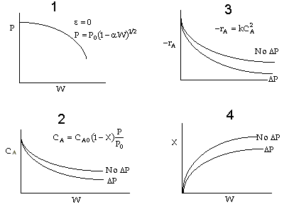
\( y = (1 - \alpha W)^{1/2} \)
CAUTION: Never use this form if \( \epsilon \neq 0 \)
For \( \epsilon = 0 \):
\( C_A = C_{A0}(1 - X)p = C_{A0}(1 - X)(1 - \alpha W)^{\frac{1}{2}} \)
Combine:
\( -r_A' = kC_A^2 = kC_{A0}^2(1 - X)^2(1 - \alpha W) \)
\( F_{A0} \frac{dX}{dW} = -r_A' \)
\( \frac{dX}{dW} = \frac{kC_{A0}^2}{F_{A0}}(1 - X)^2(1 - \alpha W) \)
Solve:
\( \frac{X}{1 - X} = \frac{kC_{A0}^2}{F_{A0}} \left[ W - \frac{\alpha W^2}{2} \right] \)
Could now solve for X given W, or for W given X.
For gas phase reactions, as the pressure drop increases, the concentration decreases,
resulting in a decreased rate of reaction, hence a lower conversion when compared to a
reactor without a pressure drop.
Here are some links to example problems dealing with packed bed reactors. You could
also use these problems as self tests.
Analysis using Simulation Tools
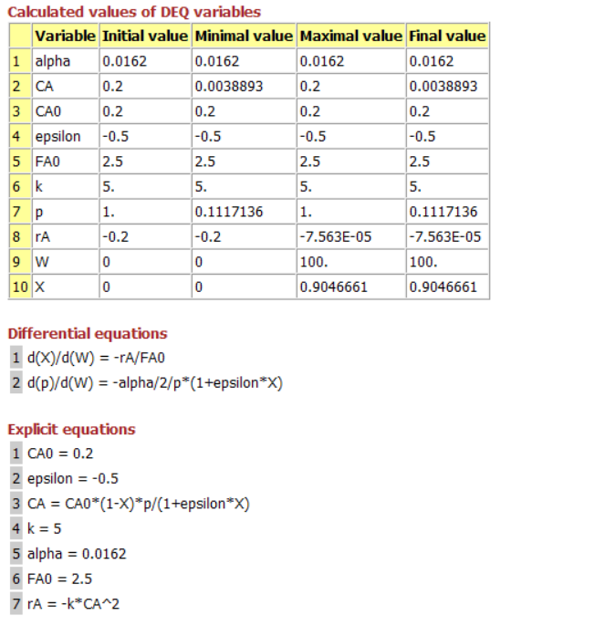
Consider the following gas phase reaction carried out isothermally in a packed bed reactor containing 100 kg of catalyst. Pure A is fed at a rate of 2.5 mol/s and with $ {C_{A0} = 0.2 \frac{mol}{dm^3}} $, and $ {\alpha = 0.0162kg^{-1}} $.
\( 2A \rightarrow B \)
Mole Balance
$ {\frac{dX}{dW} = -r_A^{'} / F_{A0}} $
Rate Law
Elementary: $ {r_A^{'} = -kC_A^2} $
Stoichiometry
Gas with ${T = T_0}$
${A \rightarrow \frac{1}{2}B \\ C_A = \frac{F_A}{v} = \frac{C_{A0}(1-X)p}{1+\epsilon X} \\ \frac{dp}{dW} = -\alpha \frac{1+\epsilon X}{2p} \\ \epsilon = -1/2 \\ F_{A0} = 2.5 \\ C_{A0} = 0.2 \\ k = 5 \\ \alpha = 0.0162 \\ W_{final} = 100 \\ X(W = 0) = 0, p(W = 0) = 1 }$
The above equations can be easily combined with the help of simulation tools such as Polymath, Wolfram or Python.
Below is the result from Polymath
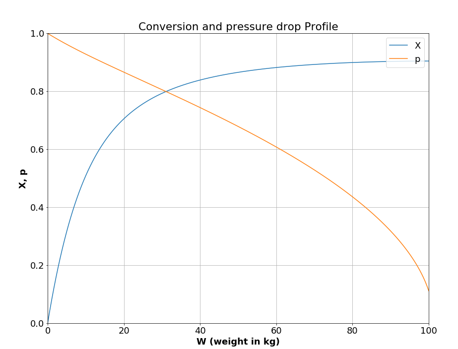
Here are links to Polymath, Wolfram, and Python code for the above example
Polymath CodeWolfram Code
Python Code
Optimum Particle Diameter
\( A \rightarrow B \)
\( -r_A = kC_{A0}(1 - X)p, \, p = \frac{P}{P_0} \)
\( \frac{dp}{dW} = -\frac{\alpha}{2p}(1 + \epsilon X) \)
as \( \alpha \) increases the pressure drop increases
\( \alpha = \frac{2G}{A_c \rho_c P_0 \rho_0 D_P \phi^3} \left[ \frac{150(1 - \phi)\mu}{D_P} + 1.75G \right] \)
Laminar Flow, Fix \( P_0, \rho_0, \phi \)
\( \rho_0 = \frac{P_0 (\text{MW})}{RT_0} \)
\( \rho_0 P_0 \sim P_0^2 \)
\( \alpha \sim \frac{G}{A_C D_P^2 P_0^2} \)
\( \alpha_2 = \alpha_1 \left( \frac{G_2}{G_1} \right) \left( \frac{D_{P1}}{D_{P2}} \right)^2 \left( \frac{A_{C1}}{A_{C2}} \right) \left( \frac{P_{01}}{P_{02}} \right)^2 \)
If \( D_{P2} = 2D_{P1}, \, G_1 = G_2, \, A_{C1} = A_{C2} \)
\( \alpha_2 = \alpha_1 \left( \frac{1}{2} \right)^2 = \frac{\alpha_1}{4} \)
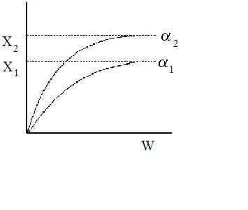
Increasing the particle diameter descreases the pressure drop and increases the rate and conversion.
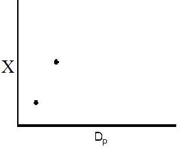
However, there is a competing effect. The specific reaction rate decreases as the particle size increases, therefore so deos the conversion.
k ∼ 1/Dp
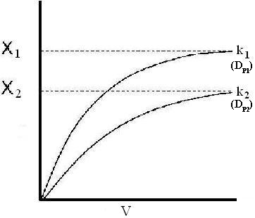
DP1 > DP2
k1 > k2
Higher k, higher conversion

The larger the particle, the more time it takes the reactant to get in and out of the catalyst particle. For a given catalyst weight, there is a greater external surgace area for smaller particles than larger particles. Therefore, there are more entry ways into the catalyst particle.
Later on in the course, we will learn that effectiveness factor decreases as the particle size increases
Engineering Analysis - Critical Thinking and Creative Thinking
TopWe want to learn how the various parameters (particle diameter, porosity, etc.) affect the pressure drop and hence conversion. We need to know how to respond to "What if" questions, such as:
"If we double the particle size, decrease the porosity by a factor of 3, and double the pipe size, what will happen to D P and X?"
(See Critical Thinking in Preface Table P1 and P2 on pages xvi and xvii. e.g., Questions the probe consenquences)
To answer these questions we need to see how a varies with these parameters.
\( \alpha = \frac{2G}{A_C \rho_0 \rho_c g_c D_P \phi^3 P_0} \left[ \frac{150 \mu (1 - \phi)}{D_P} + 1.75G \right] \)
Turbulent Flow
\( \alpha \sim \frac{G^2}{A_c D_P P_0^2} \)
Compare Case 1 and Case 2:
For example, Case 1 might be our current situation and Case 2 might be the parameters we want to change to.
\( \boxed{\alpha_2 = \alpha_1 \left( \frac{G_2}{G_1} \right)^2 \left( \frac{A_{c1}}{A_{c2}} \right) \left( \frac{D_{P1}}{D_{P2}} \right) \left( \frac{P_{01}}{P_{02}} \right)^2} \)
For constant mass flow through the system, \( \dot{m} = \text{constant} \)
\( A + \frac{1}{2} B \rightarrow \frac{1}{2} C \)
Laminar Flow
\( \alpha \sim \frac{G}{A_c D_P^2}, \quad G = \frac{\dot{m}}{A_c} \)
\( \alpha_2 = \alpha_1 \left(\frac{D_{P1}}{D_{P2}}\right)^2 \left(\frac{A_{c1}}{A_{c2}}\right)^2 \)
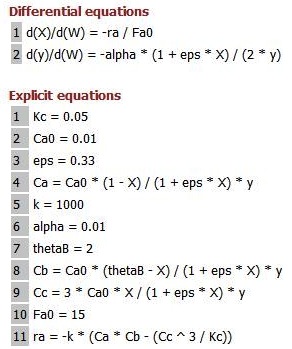
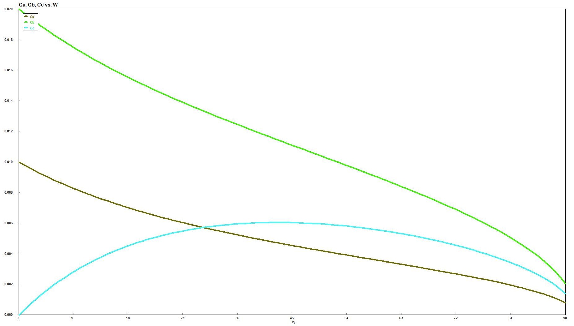
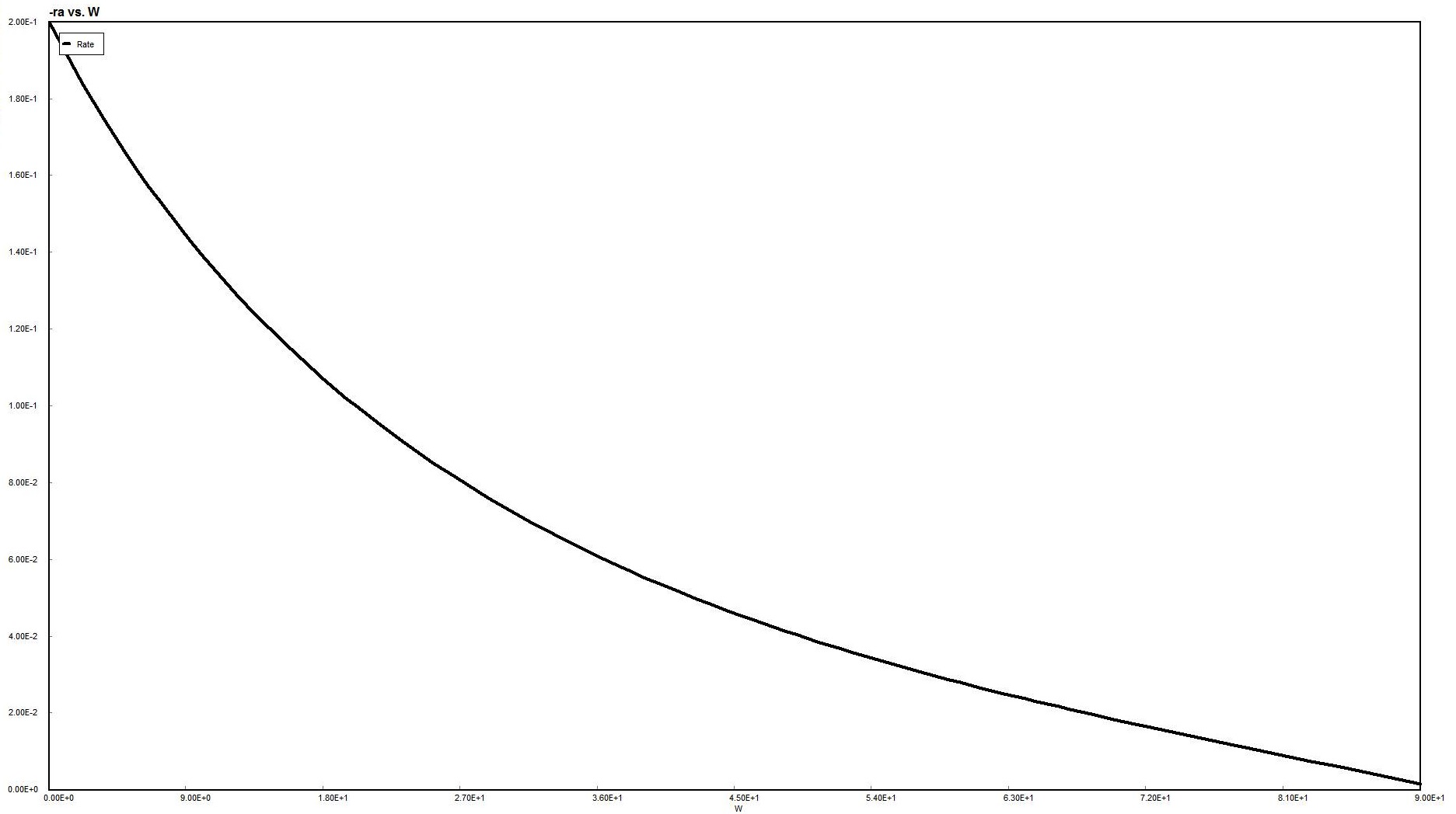
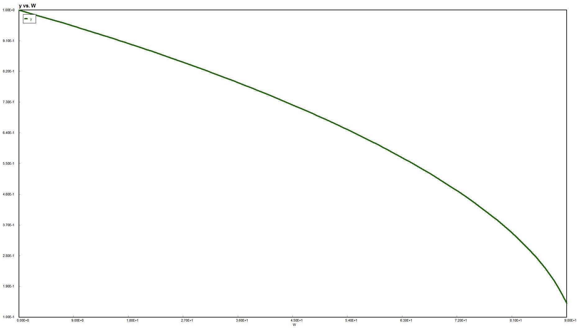
Polymath Book Problem
The following is an example problem from the book. It is located on page 192 in Chapter 5. This is a problem done in polymath and the .pol file has been included for reference. The report and accompanying graphs generated in Polymath are also shown.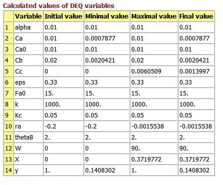
Here are more links to example problems dealing with packed bed reactors. Again, you could
also use these problems as self tests.
* All chapter references are for the 1st Edition of the text Essentials of Chemical Reaction Engineering .
