Chapter 3: Rate Laws
Rationale For Chapter 3
In chapter 2 we saw that if we had –rA as a function of X, [–rA= f(X)] we could size many reactors and reactor sequences and systems.
|
How do we obtain –rA = f(X)? We do this in two steps 1. Part 1 - Chapter 3 Rate Law – Find the rate as a function of concentration, –rA = k fn (CA, CB …) 2. Part 2 - Chapter 4 Stoichiometry – Find the concentration as a function of conversion CA = g(X) Combine Part 1 and Part 2 to get -rA=f(X) |
Rate Laws
A rate law describes the behavior of a reaction. The rate of a reaction is a function of temperature (through the rate constant) and concentration.
Topics
- Relative Rates of Reaction
- Power Law Model
- Rate Constant, k
- Elementary Reactions
- Non-Elementary Rate Laws
- Reversible Reactions
Relative Rates of Reaction
Top\( aA + bB \rightarrow cC + dD \)
Example Relative Rates of ReactionA0 and FA0
Power Law Model
Top\[-r_A = kC_A^{\alpha}C_B^{\beta}\]
\(\alpha \text{ order in A}\)
\(\beta \text{ order in B}\)
\(\text{Overall Reaction Order} = \alpha + \beta\)
The following table contains rate laws that were found experimentally.
| Reaction | Rate Law |
|---|---|
| A. First-Order Rate Laws | |
| \(C_2H_6 \rightarrow C_2H_4 + H_2\) | \(-r_A = kC_{C_2H_6}\) |
| \(\phi N = NCl \rightarrow \phi Cl + N_2\) | \(-r_A = kC_{\phi N=NCl}\) |
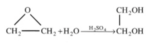
|
\(\ce{CH2OCH2 + H2O ->[H2SO4] HOCH2CH2OH}\) |
\(-r_A = kC_{CH_2OCH_2}\) |
| \(CH_3COCH_3 \rightarrow CH_2CO + CH_4\) | \(-r_A = kC_{CH_3COCH_3}\) |
| \(nC_4H_{10} \leftrightarrow iC_4H_{10}\) | \(-r_n = k\left(C_{nC_4} - \frac{C_{iC_4}}{K_C}\right)\) |
| B. Second-Order Rate Laws | |
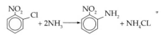
|
\(\ce{C6H4(NO2)Cl + 2NH3 -> C6H4(NO2)NH2 + NH4Cl}\) |
\(-r_A = k_{ONCB}C_{ONCB}C_{NH_3}\) |
| \(CNBr + CH_3NH_2 \rightarrow CH_3Br + NCNH_2\) | \(-r_A = kC_{CNBr}C_{CH_3NH_2}\) |
| \(CH_3COOC_2H_5 + C_4H_9OH \leftrightarrow CH_3COOC_4H_9 + C_2H_5OH\) | \(-r_A = k\left(C_AC_B - \frac{C_CC_D}{K_C}\right)\) |
| C. Non-elementary Rate Laws | |
| \(CH_3CHO \rightarrow CH_4 + CO\) | \(-r_{CH_3CHO} = kC_{CH_3CHO}^{3/2}\) |
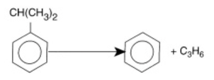
|
\(\ce{C6H5CH(CH3)2 -> C6H6 + C3H6}\) Cumene (\(C\)) → Benzene (\(B\)) + Propylene (\(P\)) |
\[ -r_C = \frac{k\left(P_C - P_BP_P/K_P\right)}{1 + K_BP_B + K_CP_C} \] |
| D. Enzymatic Reactions (Urea (U) + Urease (E)) | |
| \(NH_2CONH_2 + H_2O + Urease \rightarrow 2NH_3 + CO_2 + Urease\) | \(-r_U = \frac{kC_U}{K_M + C_U}\) |
| E. Biomass Reactions | |
| Substrate (\(S\)) + Cells (\(C\)) → More Cells + Product | \(-r_U = \frac{kC_SC_C}{K_S + C_S}\) |
Note: The rate constant, \(k\), and activation energies for a number of the reactions in these examples are given in the Data Base on the CD-ROM and Summary Notes.
Rate Constant, k
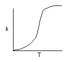
Topk is the specific reaction rate (constant) and is given by the Arrhenius Equation:
 |
\(T \to \infty\) | \(k \to A\) | \(T \to 0\) | \(k \to 0\) | \(A \approx 10^{13}\) |
\(\mathbf{k = A e^{-\frac{E}{RT}}}\)
E = activation energy (cal/mol)
R = gas constant (cal/mol*K)
T = temperature (K)
A = frequency factor (units of A, and k, depend on overall reaction order)
\(\ln k = \ln A - \frac{E}{R} \left(\frac{1}{T}\right)\)
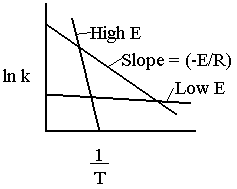
The larger the activation energy, the more temperature sensitive k and thus the reaction rate.
\(k(T_2) = k(T_1) \exp\left[\frac{E}{R} \left(\frac{1}{T_1} - \frac{1}{T_2}\right)\right]\)
Why is there an Activation Energy?
- the molecules need energy to distort or stretch their bonds in order to break them and to thus form new bonds
- as the reacting molecules come close together they must overcome both steric and electron repulsion forces in order to react
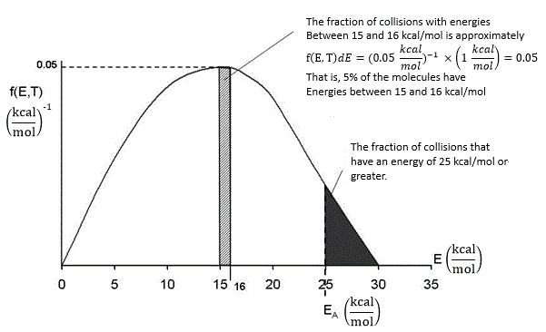
In our development of collision theory we assumed all molecules had the same average energy. However, all the molecules don’t have the same energy, rather there is distribution of energies where some molecules have more energy than others. The distraction function f(E,T) describes this distribution of the energies of the molecules. The distribution function is read in conjunction with dE
\(f(E, T)\,dE = \text{fraction of molecules with energies between } E \text{ and } E + dE\)
One such distribution of energies is in the following figure.
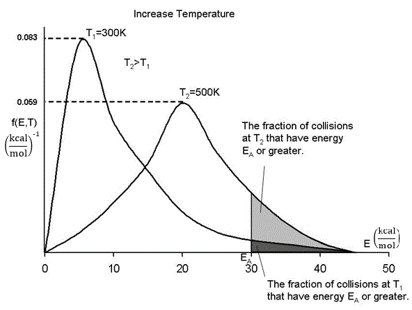
By increasing the temperature we increase the kinetic energy of the reactant molecules which can in turn be transferred to internal energy to increase the stretching and bending of the bonds causing them to be in an activated state, vulnerable to bond breaking and reaction.
We see that as the temperature is increased we have greater number of molecules have energies E A or greater and hence the reaction rate will be greater.
You can tell the overall reaction order by the units of k
| \(C_A\) | \(-r_A\) | Reaction Order | Rate Law | \(k\) |
|---|---|---|---|---|
| (mol/dm3) | (mol/dm3·s) | Zero | \(-r_A = k\) | (mol/dm3·s) |
| (mol/dm3) | (mol/dm3·s) | First | \(-r_A = kC_A\) | s-1 |
| (mol/dm3) | (mol/dm3·s) | Second | \(-r_A = kC_A^2\) | (dm3/mol·s) |
The activation energy is a "measure" of the energy a that the reacting molecules must have in order for the reaction to occur.

The reaction of AB + C to form A + BC is shown above along the reaction coordinate. One way to think of the reaction coordinate is the linear distance between the AB molecule for a fixed linear distance between the AC molecule. At the start of the reaction the AB distance is small and the BC distance is large. As the reaction proceeds, the A–C distance remains fixed but B moves away for A and closer to C and the energy of system increases. At the top of the barrier molecule B is equal distance from A and C. But as it crosses the barrier it moved close to C to form the BC molecule and the A molecule alone.
Elementary Rate Laws
TopA reaction follows an elementary rate law if and only if the (iff) stoichiometric coefficients are the same as the individual reaction order of each species. For the reaction in the previous example \(\left( A + B \rightarrow C + D \right)\), the rate law would be: \(-r_A = kC_A C_B\)
Example: If the reaction is \(2\text{NO} + \text{O}_2 \rightarrow 2\text{NO}_2\), then elementary the rate would be \(-r_{\text{NO}} = k_{\text{NO}} (C_{\text{NO}})^2 C_{\text{O}_2}\)
Non-Elementary Rate Laws
TopExample: If the rate law for the non-elementary reaction \(\left( A + B \rightarrow C + D \right)\) is found to be \(-r_A = kC_A^2C_B\)
Then the reaction is said to be 2nd order in A, 1st order in B, and 3rd order
overall.
Reversible Reactions
TopThe net rate of formation of any species is equal to its rate of formation in the forward reaction plus its rate of formation in the reverse reaction:
\(\text{rate}_{\text{net}} = \text{rate}_{\text{forward}} + \text{rate}_{\text{reverse}}\)
At equilibrium, \(\text{rate}_{\text{net}} \stackrel{\text{eq}}{\approx} 0\)
and the rate law must reduce to an equation that is thermodynamically consistent
with the equilibrium constant for the reaction.
Example: Consider the exothermic, heterogeneous reaction \(A + B \rightarrow C\)
At low temperature, the rate law for the disappearance of A is
\(-r'_A = \frac{k_A P_A P_B}{1 + K_A P_A}\) (Recall \(P_A = C_A R T\))
At high temperature, the exothermic reaction is significantly reversible: \(\text{A} + \text{B} \rightleftharpoons \text{C}\)
What is the corresponding rate law? Let's see.
If the rate of formation of A for the forward reaction (\(\text{A} + \text{B} \longrightarrow \text{C}\)) is
\[r'_{A\text{for}} = \frac{-k_A P_A P_B}{1 + K_A P_A}\]
then we need to assume a form of the rate law for the reverse reaction that satisfies the equilibrium condition.
If we assume the rate law for the reverse reaction (\(\text{C} \rightarrow \text{A} + \text{B}\)) is:
\[r'_{{A,\text{rev}}} = \frac{k_{-A} P_C}{1 + K_A P_A}\]
then: \[r_A = r_{A,\text{net}} = r_{A,\text{for}} + r_{A,\text{rev}}\]
and: \[-r'_A = \frac{k_A}{1 + K_A P_A} \left(P_A P_B - \frac{P_C}{K_P}\right)\]
Does this rate law satisfy our requirement that, at equilibrium, it must reduce to an equation that is thermodynamically consistent with KP? Let's see.
From Appendix C we know that for a reaction at equilibrium:
\[K_P = \frac{P_{Ce}}{P_{Ae} P_{Be}}\]
At equilibrium, \(r_{\text{net}} \cong 0\), so: \[-r_A \cong 0 = \frac{k_A}{1 + K_A P_{Ae}} \left( P_{Ae} P_{Be} - \frac{P_{Ce}}{K_P} \right)\]
Solving for KP gives:
\[K_P = \frac{P_{Ce}}{P_{Ae} P_{Be}}\]
The conditions are satisfied.
Useful Links
Top* All chapter references are for the 1st Edition of the text Essentials of Chemical Reaction Engineering .