Chapter 11: Nonisothermal Reactor Design: The Steady State Energy Balance and Adiabatic PFR Applications
Topics
- Why Use the Energy Balance?
- Overview of User Friendly Energy Balance Equations
- Manipulating the Energy Balance, DHRx
- Reversible Reactions
- Adiabatic Reactions
- Interstage Cooling/Heating
Energy Balances, Rationale and Overview
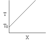
TopLet's calculate the volume necessary to achieve a conversion, X, in a PFR for a first-order, exothermic reaction carried out adiabatically. For an adiabatic, exothermic reaction the temperature profile might look something like this:
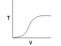
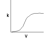
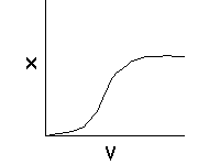
The combined mole balance, rate law, and stoichiometry yield:
| \( \frac{dX}{dV} = \frac{-r_A}{F_{A0}} \) |
| \( r_A = -k_i \exp\left[ \frac{E}{R} \left( \frac{1}{T_1} - \frac{1}{T} \right) \right] C_A \) |
| \( \frac{dX}{dV} = \frac{k_i \exp\left[ \frac{E}{R} \left( \frac{1}{T_1} - \frac{1}{T} \right) \right]}{F_{A0}} C_A (1 - X) \) |
To solve this equation we need to relate X and T.
We will use the Energy Balance to relate X and T. For example, for an adiabatic reaction, e.g.,\( A -> B\), in which no inerts the energy balance yields
\( T = T_0 + \frac{(-\Delta H_{rx}) X}{C_{P_A}} \)
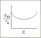
We can now form a table like we did in Chapter 2,
choose \(X\) \(\xrightarrow{\text{calculate}}\) \(T\) \(\xrightarrow{\text{calculate}}\) \(k\) \(\xrightarrow{\text{calculate}}\) \(K_c\) \(\xrightarrow{\text{calculate}}\) \(-r_A\) \(\xrightarrow{\text{calculate}}\) \(\left( \frac{F_{A0}}{-r_A} \right)\) increment \(X\) and repeat
User Friendly Energy Balance Equations
TopThe user friendly forms of the energy balance we will focus on are outlined in the following table.
|
User friendly equations relating X and T, and Fi and T 1. Adiabatic CSTR, PFR, Batch, PBR achieve this:
2. CSTR with heat exchanger, UA(Ta-T) and large coolant flow
rate.
3A. In terms of conversion, X
3B. In terms of molar flow rates, Fi
4. For Multiple Reactions
5. Coolant Balance
|
||||||||||||||
|
These equations are derived in the text. These are the equations that we will use to solve reaction engineering problems with heat effects. |
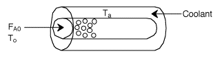
Energy Balance
TopIn the material that follows, we will derive the above equations.
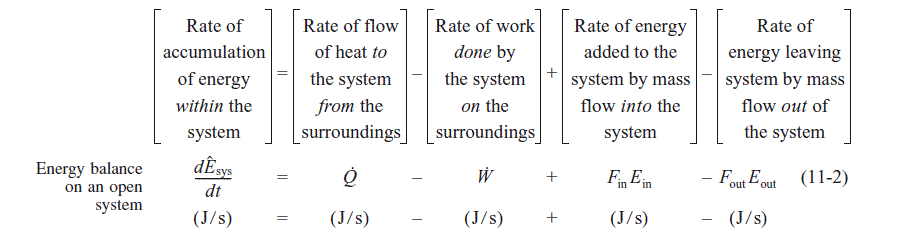
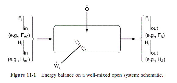
We need to put the above equation into a form that we can easily use to relate X and T in order to size reactors. To achieve this goal, we write the molar flow rates in terms of conversion and the enthalpies as a function of temperature. We now will "dissect" both Fi and Hi. [Note: For an animated derivation of the following equations, see the Interactive Computer Modules (ICMs) Heat Effects 1 and Heat Effects 2.]
|
Flow Rates, Fi |
||
|
For the generalized reaction: \( A + \frac{b}{a} B \rightarrow \frac{c}{a} C + \frac{d}{a} D \) |
||
|
\( F_A = F_{A0} (1 - X), \quad F_B = F_{A0} \left( \frac{b}{a} - \frac{b}{a} X \right) \) In general, \( F_i = F_{A0} \left( \nu_i + \nu_i X \right) \) |
||
| \( \nu_A = -1, \quad \nu_B = -\frac{b}{a}, \quad \nu_C = \frac{c}{a}, \quad \nu_D = \frac{d}{a} \) | ||
|
Assuming no phase change: |
||
| \( H_i = H_i^\circ (T_R) + \int_{T_R}^{T} C_{p,i} dT \) | ||
| \( \sum_i H_i = \Delta H_R (T) = \Delta H_R^\circ (T_R) + \int_{T_R}^{T} \Delta C_p dT \) | ||
| \( \Delta H_{RX} = \frac{d}{a} H_D + \frac{c}{a} H_C - \frac{b}{a} H_B - H_A \) | ||
| \( \Delta C_p = \frac{d}{a} C_{pD} + \frac{c}{a} C_{pC} - \frac{b}{a} C_{pB} - C_{pA} \) | ||
| \( C_{p,i} = \alpha_i + \beta_i T + \chi_i T^2 \) | ||
|
|
||
| \( \hat{C}_{p,i} = \int_{T_R}^{T} C_{p,i} \, dT \) | \( \tilde{C}_{p,i} = \frac{T_{io}}{(T - T_{io})} \) | |
| \( H_i = H_i^\circ(T_R) + \hat{C}_{p,i}(T - T_R) \) | \( \Delta H_R(T) = \Delta H_R^\circ(T_R) + \hat{C}_p(T - T_R) \) | |
| \( \sum_u \hat{C}_{p,i} = \Delta C_p = \frac{d}{a} \hat{C}_{p,FD} + \frac{c}{a} \hat{C}_{p,FC} - \frac{b}{a} \hat{C}_{p,FB} - \hat{C}_{p,FA} \) | ||
|
|
||
| \( \dot{Q} - \dot{W}_s - F_{A0} \int_{T_R}^{T} \sum_u \hat{C}_{p,i} dT - F_{A0} X \left[ \Delta H_R^\circ(T_R) + \int_{T_R}^{T} \Delta C_p dT \right] = 0 \) | ||
|
|
||
| \( \dot{Q} - \dot{W}_s - F_{A0} X \left[ \Delta H_R^\circ(T_R) + \Delta C_p (T - T_R) \right] = F_{A0} \sum_u \hat{C}_{p,i} (T - T_0) \) | ||
|
Adiabatic Energy Balance: |
\( T = T_0 - \frac{X \left[ \Delta H_R^\circ(T_R) + \Delta C_p (T_0 - T_R) \right]}{\sum_u \hat{C}_{p,i} + X \Delta C_p} = T_0 - \frac{X \left[ \Delta H_R(T) \right]}{\sum_u \hat{C}_{p,i} + X \Delta C_p} \) |
|
|
|
Adiabatic Energy Balance for variable heat capacities: |
|
| \( X = \frac{\sum_u \alpha_i (T_0 - T) + \frac{1}{2} \sum_u \beta_i
(T_0^2 - T^2) + \frac{1}{3} \sum_u \gamma_i (T_0^3 - T^3)}{\Delta H_{RX} (T_R) +
\Delta \alpha (T - T_R) + \frac{1}{2} \Delta \beta (T^2 - T_R^2) + \frac{1}{3}
\Delta \gamma (T^3 - T_R^3)} \)
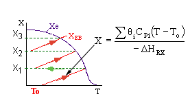
For constant heat capacities: \( \beta = \gamma = 0, \ \alpha = C_{pi} \) \( X = \frac{\sum_u \theta_i C_{pi} (T - T_0)}{-\Delta H_{RX}} \) We will only be considering constant heat capacities for now. |
|
Reversible Reactions
TopConsider the reversible gas phase elementary reaction.
\( A \rightleftharpoons B \)
The rate law for this gas phase reaction will follow an elementary rate law.
\( -r_A = k \left[ C_A - \frac{C_B}{K_c} \right] \)
Where Kc is the concentration equilibrium constant. We know from Le Chaltlier's Law that if the reaction is exothermic, Kc will decrease as the temperature is increased and the reaction will be shifted back to the left. If the reaction is endothermic and the temperature is increased, Kcwill increase and the reaction will shift to the right.
at equilibrium
\( -r_A = 0 \)
\( K_c = \frac{C_{B\beta}}{C_{A\beta}} = \frac{C_{A0} X_\beta \frac{T_0}{T} p}{C_{A0} (1 - X_\beta) \frac{T_0}{T} p} = \frac{X_\beta}{1 - X_\beta} \)
\( X_\beta = \frac{K_c}{1 + K_c} \)
\( K_c = \frac{K_P}{(RT)^\delta} \)
Van't Hoff Equation
\( \frac{d \ln K_P}{dT} = \frac{\Delta H_R(T)}{RT^2} = \frac{\Delta H_R^\circ(T_R) + \Delta \hat{C}_P (T - T_R)}{RT^2} \)
For the special case of \( \Delta \hat{C}_P = 0 \)
Integrating the Van't Hoff Equation gives:
\( K_P(T_2) = K_P(T_1) \exp \left[ \frac{\Delta H_R^\circ(T_R)}{R} \left( \frac{1}{T_1} - \frac{1}{T_2} \right) \right] \)
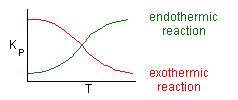
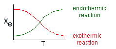
\( \delta = 0 \)
\( K_c(T) = K_c(T_1) \exp \left[ \frac{\Delta H_{RX}}{R} \left( \frac{1}{T_1} - \frac{1}{T} \right) \right] \)
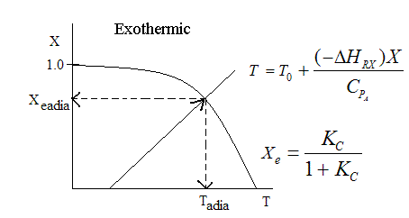
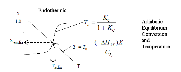
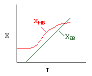
Adiabatic Equilibrium
Conversion on Temperature
Exothermic ΔH is negative
Adiabatic Equilibrium temperature (Tadia) and conversion (Xeadia
Endothermic ΔH is positive
Adiabatic Reactions
TopAlgorithm Adiabatic Reactions:
Suppose we have the Gas Phase Reaction
\( A \rightleftharpoons 2B \)
that follows an elementary rate law. To generate a Levenspiel plot to size CSTRs and PFRs we use the following steps or as we will see later use POLYMATH.
| 1. Choose X | |
| Calculate T | \( T = T_0 - \frac{\Delta H_{rx} X}{\sum \theta_i C_{pi}} \) |
| Calculate k | \( k = k_1 \exp \left( \frac{E}{R} \left( \frac{1}{T_1} - \frac{1}{T} \right) \right) \) |
| Calculate KC | \( K_c = K_{c2} \exp \left( \frac{\Delta H_{rx}}{R} \left( \frac{1}{T_2} - \frac{1}{T} \right) \right) \) |
| Calculate To/T | |
| Calculate CA | \( C_A = \frac{C_{A0}(1 - X)}{1 + \epsilon X} \left( \frac{T_0}{T} \right) \) |
| Calculate CB | \( C_B = \frac{C_{A0} X}{1 + \epsilon X} \left( \frac{T_0}{T} \right) \) |
| Calculate -rA | \( -r_A = k \left( C_A - \frac{C_B^2}{K_c} \right) \) |
| 2. Increment X and then repeat calculations. | |
| 3. When finished, plot \( \frac{F_{A0}}{-r_A} \) vs. X or use some numerical technique to find V. | |
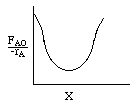 Levenspiel Plot for an exothermic, adiabatic reaction.
We can now use the techniques developed in Chapter 2 to size reactors and reactors in series to compare and size CSTRs and PFRs. |
|
|
Consider:
CSTR: \( V_1 = \frac{F_{A0}}{-r_A} X_1 \)
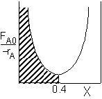
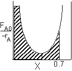
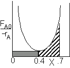
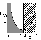
PFR: \( V_1 = \int_0^{X_1} \frac{F_{A0}}{-r_A} dX \)
|
|
|
 PFR
Shaded area is the volume.
PFR
Shaded area is the volume. |
||
|
For an exit conversion of 40% |
For an exit conversion of 70% |
|
|
|
|
|
CSTR
|
||
|
For an exit conversion of 40% |
For an exit conversion of 70% |
|
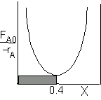
|
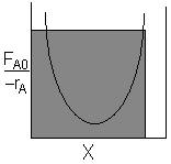
|
|
|
We see for 40% conversion very little volume is required. CSTR+PFR |
||
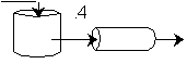
|
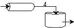
|
|
| (a) | (b) | |
|
For an intermediate conversion of 40% and exit conversion of 70% |
||
|
|
|
| (a) | (b) | |
 Shaded
area is
the
reactor volume.
Shaded
area is
the
reactor volume.Looks like the best arrangement is a CSTR with a 40% conversion followed by a PFR up to 70% conversion.
Interstage Cooling/Heating
Top|
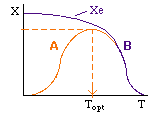
Curve A: Reaction rate slow, conversion dictated by rate of
reaction and
reactor
volume. As temperature increases rate increases and therefore
conversion
increases. |
||
|
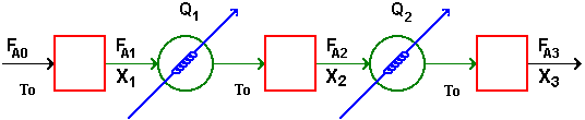
Interstage Cooling: |
||
|
||
|
||
CSTR Algorithm
|
1.) |
Given X |
|
|
2.) |
Given T |
|
|
3.) |
Given V |
|
|
||