Chapter 7: Collection and Analysis of Rate Data
Finding the Rate Law
Consider the following reaction that occurs in a constant volume batch reactor: (We will withdraw samples and record the concentration of A as a function of time.)
A \(\rightarrow\) Products
Mole Balance:
\(\frac{dN_A}{dt} = r_A V\)
Rate Law:
\(-r_A = k C_A^\alpha\)
Stoichiometry:
\(V = V_0\)
Combine:
\(\frac{dC_A}{dt} = k C_A^\alpha\)
Topics
Integral Method
TopWe could integrate the combined mole balance and rate law to plot reaction rate data in terms of
concentration vs. time for 0, 1st, and 2nd order reactions.
Table 7.1- Derivation Equations used to Plot 0,
1st, and 2nd order reactions.
These types of plots are usually used to determine the values k for runs at various
temperatures and then used to determine the activation energy.
| Zero Order | First Order | Second Order |
|---|---|---|
|
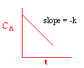
Zero order, \(\alpha = 0\) |
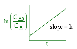
First order, \(\alpha = 1\) |
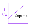
Second order, \(\alpha = 2\) |
|
|
|
|
Equation: \( \frac{dC_A}{dt} = r_A = -k \) At \( t = 0 \), \( C_A = C_{A0} \) Solution: \( C_A = C_{A0} - kt \) |
Equation: \( \frac{dC_A}{dt} = r_A = -kC_A \) At \( t = 0 \), \( C_A = C_{A0} \) Solution: \( \ln{\left( \frac{C_{A0}}{C_A} \right)} = kt \) |
Equation: \( \frac{dC_A}{dt} = r_A = -kC_A^2 \) At \( t = 0 \), \( C_A = C_{A0} \) Solution: \( \frac{1}{C_A} - \frac{1}{C_{A0}} = kt \) |
If the data do not fall on a straight line for α=0,1, or 2 such as α=2;
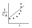
then we should stop guessing reaction orders and proceed to either the differential method of analysis or to regression.
Differential Method
TopTaking the natural log of \(\frac{dC_A}{dt} = k C_A^\alpha\),
\(\ln \left( - \frac{dC_A}{dt} \right) = \ln k + \alpha \ln C_A\)
The reaction order can be found from a ln-ln plot of:
\(\left( - \frac{dC_A}{dt} \right) \, \text{vs} \, C_A\)
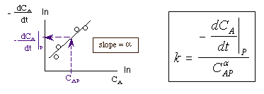
Methods for finding the slope of log-log and semi-log graph papers may be found at http://www.physics.uoguelph.ca/tutorials/GLP/.
However, we are usually given concentration as a function of time from batch
reactor experiments.
| Time (s) | 0 | t1 | t2 | t3 |
|---|---|---|---|---|
| Concentration (mol/dm3) | CA0 | CA1 | CA2 | CA3 |
Three Ways to Determine (-dCA/dt) from Concentration-Time Data (Graphical, Polynomial, Finite Difference, Non-Linear Least Squares Analysis)
2A. Graphical
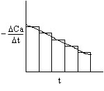
This method accentuates measurement error!
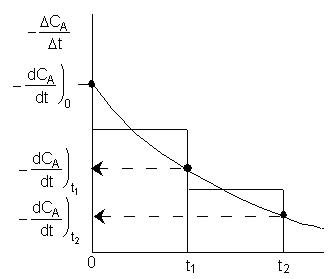
2B. Polynomial (using Polymath)
\(C_A = a_0 + a_1 t + a_2 t^2 + a_3 t^3 + a_4 t^4\)
\(\frac{dC_A}{dt} = a_1 + 2a_2 t + 3a_3 t^2 + 4a_4 t^3\)
2C. Finite Difference
\(\frac{dC}{dt}\Bigg|_i = \frac{C_{i+1} - C_{i-1}}{2 \Delta t}\)
Non-Linear Least-Squares Analysis
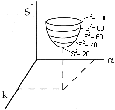
TopWe want to find the parameter values (alpha, k, E) for which the sum of the squares of the differences, the measured parameter (Pm), and the calculated parameter (Pc) is a minimum.
\(\sigma^2 = \frac{\sum_{i=1}^{n} (P_{mi} - P_{ci})^2}{N - K}\)
That is we want \(\sigma^2\) to be a minimum.
| Time (s) | 0 | t1 | t2 | t3 |
|---|---|---|---|---|
| Concentration (mol/dm3) | CA0 | CA1 | CA2 | CA3 |
For concentration-time data, the measured parameter P has concentration CA. We can integrate the combined mole balance equation and rate law
\(\frac{dC_A}{dt} = - C_A^\alpha\)
to obtain
\(C_A = \left[ C_{A0}^{1-\alpha} - (1 - \alpha) k t \right]^{\frac{1}{1-\alpha}}\)
We now guess k and alpha and calculate each CACi at the times shown in the above table and then compare it with the measured concentration by taking the difference and squaring it.
We then sum up the differences for all the data points.
\( s^2 = \sum_{i=1}^{N} (C_{Ami} - C_{Aci})^2 = \sum_{i=1}^{N} \left( C_{Ami} - \left[ C_{A0}^{1-\alpha} - (1 - \alpha) k t_i \right]^{\frac{1}{1-\alpha}} \right)^2 \)
We continue to guess k and alpha until we find the values of alpha and k which minimize S2 (actually we let the computer find these values.)
* All chapter references are for the 1st Edition of the text Essentials of Chemical Reaction Engineering .