Chapter 4: Stoichiometry
Rationale For Chapter 4
In chapter 2 we saw that if we had –rA as a function of X, [–rA= f(X)] we could size many reactors and reactor sequences and systems.

|
How do we obtain –rA = f(X)? We do this in two steps 1. Part 1 - Chapter 3 Rate Law – Find the rate as a function of concentration, –rA = k fn (CA, CB …) 2. Part 2 - Chapter 4 Stoichiometry – Find the concentration as a function of conversion CA = g(X) Combine Part 1 and Part 2 to get -rA=f(X) |
Stoichiometry
We shall set up Stoichiometric Tables using A as our basis of calculation
in the following reaction. We will use the stoichiometric tables to express
the concentration as a function of conversion. We will combine Ci
= f(X) with the appropriate rate law to obtain -rA = f(X).
Topics
Batch System Stoichiometric Table
Top| Species | Symbol | Initial | Change | Remaining |
|---|---|---|---|---|
| A | A | \( N_{A0} \) | \( -N_{A0}X \) | \( N_A = N_{A0}(1 - X) \) |
| B | B | \( N_{B0} = N_{A0} \Theta_B \) | \( -\frac{b}{a} N_{A0}X \) | \( N_B = N_{A0} \left( \Theta_B - \frac{b}{a} X \right) \) |
| C | C | \( N_{C0} = N_{A0} \Theta_C \) | \( +\frac{c}{a} N_{A0}X \) | \( N_C = N_{A0} \left( \Theta_C + \frac{c}{a} X \right) \) |
| D | D | \( N_{D0} = N_{A0} \Theta_D \) | \( +\frac{d}{a} N_{A0}X \) | \( N_D = N_{A0} \left( \Theta_D + \frac{d}{a} X \right) \) |
| Inert | I | \( N_I = N_{A0} \Theta_I \) | – | \( N_I = N_{A0} \Theta_I \) |
| \( N_{T0} \) | \( N_T = N_{T0} + \delta N_{A0}X \) | |||
Where:
\(
\Theta_i = \frac{N_{i0}}{N_{A0}} = \frac{C_{i0}}{C_{A0}} = \frac{Y_{i0}}{Y_{A0}} \quad \text{and} \quad \delta = \frac{d}{a} + \frac{c}{a} - \frac{b}{a} - 1
\)
|
Concentration -- Batch System: \( C_A = \frac{N_A}{V} \) |
Constant Volume Batch: Note: if the reaction occurs in the liquid phase or if a gas phase reaction occurs in a rigid (e.g., steel) batch reactor, then:
\(V = V_0\)
\(C_A = \frac{N_A}{V} = \frac{N_{A0}(1 - X)}{V_0} = C_{A0}(1 - X)\)
\( C_B = \frac{N_B}{V} = \frac{N_{A0}}{V_0} \left( \Theta_B - \frac{b}{a} X \right) = C_{A0} \left( \Theta_B - \frac{b}{a} X \right) \)
etc.
if \(-r_A = k_A C_A^2 C_B\) then
|
\(-r_A = C_{A0}^3 (1 - X)^2 \left( \Theta_B - \frac{b}{a} X \right)\) |
Constant Volume Batch |
and we have -rA=f(x)
Flow System Stoichiometric Table
Top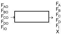
| Species | Symbol | Reactor Feed | Change | Reactor Effluent |
|---|---|---|---|---|
| A | A | \( F_{A0} \) | \( -F_{A0}X \) | \( F_A = F_{A0}(1 - X) \) |
| B | B | \( F_{B0} = F_{A0}\Theta_B \) | \( -\frac{b}{a} F_{A0}X \) | \( F_B = F_{A0}\left(\Theta_B - \frac{b}{a} X\right) \) |
| C | C | \( F_{C0} = F_{A0}\Theta_C \) | \( +\frac{c}{a} F_{A0}X \) | \( F_C = F_{A0}\left(\Theta_C + \frac{c}{a} X\right) \) |
| D | D | \( F_{D0} = F_{A0}\Theta_D \) | \( +\frac{d}{a} F_{A0}X \) | \( F_D = F_{A0}\left(\Theta_D + \frac{d}{a} X\right) \) |
| Inert | I | \( F_{I0} = F_{A0}\Theta_I \) | — | \( F_I = F_{A0}\Theta_I \) |
| \( F_{T0} \) | \( F_T = F_{T0} + \delta F_{A0}X \) | |||
Where:
\( \Theta_i = \frac{F_{i0}}{F_{A0}} = \frac{C_{i0} u_0}{C_{A0} u_0} = \frac{C_{i0}}{C_{A0}} = \frac{y_{i0}}{y_{A0}} \quad \text{and} \quad \delta = \frac{d}{a} + \frac{c}{a} - \frac{b}{a} - 1 \)
|
Concentration -- Flow System: \( C_A = \frac{F_A}{u} \) |
|
Liquid Phase Flow System: \( u = u_0 \) |
|
\( C_A = \frac{F_A}{u} = \frac{F_{A0}(1 - X)}{u_0} = C_{A0}(1 - X) \) Flow Liquid Phase \( C_B = \frac{F_B}{u} = \frac{F_{A0}}{u_0} \left( \Theta_B - \frac{b}{a} X \right) = C_{A0} \left( \Theta_B - \frac{b}{a} X \right) \) |
etc.
If the rate of reaction were -rA = kCACB then
we would have
\(
-r_A = k C_{A0}^2 (1 - X) \left( \Theta_B - \frac{b}{a} X \right)
\)
This gives us -rA = f(X). Consequently, we can use the methods
discussed in Chapter 2 to size a large number of reactors, either alone
or in series.
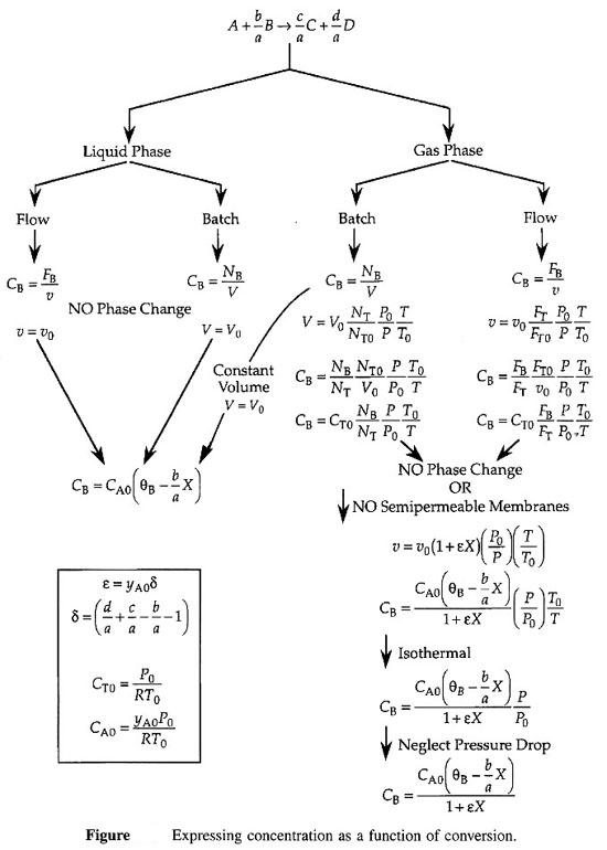
| Gas Phase Flow System: \( \upsilon = \upsilon_0 (1 + \epsilon X) \left( \frac{T}{T_0} \right) \left( \frac{P_0}{P} \right) \) |
\(C_A = \frac{F_A}{\upsilon} = \frac{F_{A0}(1 - X)}{\upsilon_0 (1 + \epsilon X)} \left(\frac{T_0}{T}\right) \left(\frac{P}{P_0}\right) = C_{A0} \left(\frac{(1 - X)}{(1 + \epsilon X)}\right) \left(\frac{T_0}{T}\right) \left(\frac{P}{P_0}\right)\)
\( C_B = \frac{F_B}{\upsilon} = \frac{F_{A0} \left( \Theta_B - \frac{b}{a} X \right)}{\upsilon_0 (1 + \epsilon X)} \left( \frac{T_0}{T} \right) \left( \frac{P}{P_0} \right) = C_{A0} \left( \frac{\Theta_B - \frac{b}{a} X}{1 + \epsilon X} \right) \left( \frac{T_0}{T} \right) \left( \frac{P}{P_0} \right) \)
etc.
Again, these equations give us information about -rA = f(X), which we can use to size reactors.
For example if the gas phase reaction has the rate law
\( -r_A = k_A C_A^2 C_B \)
then
Flow Gas Phase
\(-r_A = \frac{C_{A0}^3 (1 - X)^2 \left( \Theta_B - \frac{b}{a} X \right)}{(1 + \epsilon X)^3}\)
with
\( C_{A0} = \frac{P_{A0}}{RT} \) \( \Theta_B = \frac{y_{B0}}{y_{A0}} = \frac{C_{B0}}{C_{A0}} = \frac{F_{B0}}{F_{A0}} \)
Calculating the equilibrium conversion for gas phase reaction
Consider the following elementary reaction with KC and = 20 dm3/mol and CA0 = 0.2 mol/dm3. Pure A fed. Calculate the equilibrium conversion, Xe, for both a batch reactor and a flow reactor.
\( \text{2A} \rightleftharpoons \text{B} \)
\( -r_A = k_A \left[ C_A^2 - \frac{C_B}{K_C} \right] \)
Solution
At equilibrium
\( -r_A \equiv 0 \equiv k_A \left[ C_{Ae}^2 - \frac{C_{Be}}{K_C} \right] \)
\( K_C = \frac{C_{Be}}{C_{Ae}^2} \)
Stoichiometry
\( \text{A} \rightarrow \frac{\text{B}}{2} \)
Batch
Species Initial Change Remaining A \( N_{A0} \) \( -N_{A0}X \) \( N_A = N_{A0}(1 - X) \) B \( 0 \) \( +\frac{N_{A0}X}{2} \) \( N_B = \frac{N_{A0}X}{2} \) \( N_{T0} = N_{A0} \) \( N_T = N_{A0} - \frac{N_{A0}X}{2} \)
Constant Volume V = V0
\( C_A = \frac{N_A}{V} = \frac{N_A}{V_0} = \frac{N_{A0}(1 - X)}{V_0} = C_{A0}(1 - X) \) \( C_B = \frac{N_B}{V} = \frac{N_{A0}X/2}{V_0} = \frac{C_{A0}X}{2} \) \( K_C = \frac{C_{Be}}{C_{Ae}^2} = \frac{C_{A0} \frac{X_e}{2}}{C_{A0}^2 (1 - X_e)^2} \) \( 2K_C C_{A0} = \frac{X_e}{(1 - X_e)^2} = \left(2\right)\left(20 \, \frac{\text{dm}^3}{\text{mol}}\right)\left(0.2 \, \frac{\text{mol}}{\text{dm}^3}\right) = 8 \) \( 8X_e^2 - 17X_e + 8 = 0 \)Solving
Batch: X = 0.7
Flow
Species Fed Change Remaining A \( F_{A0} \) \( -F_{A0}X \) \( F_A = F_{A0}(1 - X) \) B \( 0 \) \( +\frac{F_{A0}X}{2} \) \( F_B = \frac{F_{A0}X}{2} \) \( F_{T0} = F_{A0} \) \( F_T = F_{A0} - \frac{F_{A0}X}{2} \)
\( C_{Ae} = \frac{C_{A0}(1 - X_e)}{1 + \varepsilon X_e} \) \( C_{Be} = \frac{C_{A0} X_e}{2 (1 + \varepsilon X_e)} \) \( K_C = \frac{\frac{C_{A0} X_e}{2 (1 + \varepsilon X_e)}}{\left(\frac{C_{A0}(1 - X_e)}{1 + \varepsilon X_e}\right)^2} = \frac{X_e (1 + \varepsilon X_e)}{2 C_{A0} (1 - X_e)^2} \) \( 2K_C C_{A0} = \frac{X_e + \varepsilon X_e^2}{1 - 2X_e + X_e^2} = 2 \left( 20 \, \frac{\text{dm}^3}{\text{mol}} \right) \left( 0.2 \, \frac{\text{mol}}{\text{dm}^3} \right) = 8 \) \( \varepsilon = y_{A0} \delta = 1 \left( \frac{1}{2} - 1 \right) = -\frac{1}{2} \) \( 8 = \frac{X_e - 0.5 X_e^2}{1 - 2 X_e + X_e^2} \) \( 8.5 X_e^2 - 17 X_e + 8 = 0 \)Flow : \(X_e = 0.757\)RecallBatch : \(X_e = 0.70\)
* All chapter references are for the 1st Edition of the text Essentials of Chemical Reaction Engineering .