After posting an example plot of my radio telescope output on the Lowbrows list, I received a couple of requests for more information. One request was for an explanation of the plot, and another was for pictures of my equipment. This brief article is in response to these requests, and I hope that it is of general interest to the rest of the club members.
My present radio telescope is an interferometer operating at about 400 MHz. It consists of two antennas separated by about 7.5 meters distance in roughly an east, west direction. The interferometer produces a distinctive cyclical pattern as a source passes through the beams of the two antennas. The interferometer has certain advantages over single antenna radio telescopes. It is primarily sensitive to small isolated sources rather than extended sources and background radiation. It is also somewhat insensitive to interference of a continuous nature such as broadcast station spurious signals.
A basic radio interferometer is depicted in Figure 1. In this diagram, many of the details have been omitted for clarity.
Signals from a source off axis by the angle ![]() produce wave-fronts
that are intercepted
by the two antennas at slightly different times. The time delay is equal
to
produce wave-fronts
that are intercepted
by the two antennas at slightly different times. The time delay is equal
to ![]() ,
where D is the baseline distance between the antennas, and c is the speed
of light.
For simplicity, it is convenient to consider monochromatic signals. The
time delay then
produces a phase difference between the two signals from the two antennas.
Each of
the antennas has a beam pattern
,
where D is the baseline distance between the antennas, and c is the speed
of light.
For simplicity, it is convenient to consider monochromatic signals. The
time delay then
produces a phase difference between the two signals from the two antennas.
Each of
the antennas has a beam pattern ![]() that modulates the signals
from the source as it
passes through the beam. The signals produced in the two feed-lines could
be approximately
modeled as:
that modulates the signals
from the source as it
passes through the beam. The signals produced in the two feed-lines could
be approximately
modeled as:
![]()
&
where V represents the voltage induced in the feed-lines by the electromagnetic field impinging on the antennas. These two signals are correlated to form the output interferogram. The correlation process is a multiplication followed by averaging or low pass filtering. The signal that results from multiplication is:

Where: ![]() The low pass filtering removes high frequency terms leaving an output
signal of the form:
The low pass filtering removes high frequency terms leaving an output
signal of the form: 
The output signal is seen to be proportional to input signal power ![]() and is modulated by the antenna power pattern
and is modulated by the antenna power pattern ![]() . It is a cosine
waveform with frequency proportional to the baseline D divided by the wavelength
. It is a cosine
waveform with frequency proportional to the baseline D divided by the wavelength
![]() .
.
The output signal would look something like the plot shown in Figure 2.
If the baseline is laid out in an east, west direction and has been accurately measured, certain information about the source can be learned from the waveforms. Assuming the antenna beam patterns are narrow enough that the center lobe of the interferogram waveform can be identified, then the source transit time (Local Mean Sidereal Time LMST) and hence its right ascension can be determined. This is done by noting the Greenwich mean sidereal time (GMST) at the peak of the central lobe. The longitude of the interferometer must, of course, also be known.
Right Ascension = GMST—Longitude/15 = LMST
It can be shown that ![]() , where
, where ![]() is the source
declination and H is the local hour angle. Since the frequency of
the cosine waveform with respect to hour angle is proportional to
declination, the declination of the source can be determined by
measuring the frequency of the interferogram. To do this precisely
requires more than simply taking a Fourier transform because the
frequency is not constant over the antenna beam pattern. Nevertheless,
the declination can be determined by least squares fitting
a mathematical model of the waveform to the output interferogram.
The third thing that can be determined is, of course, signal
power
is the source
declination and H is the local hour angle. Since the frequency of
the cosine waveform with respect to hour angle is proportional to
declination, the declination of the source can be determined by
measuring the frequency of the interferogram. To do this precisely
requires more than simply taking a Fourier transform because the
frequency is not constant over the antenna beam pattern. Nevertheless,
the declination can be determined by least squares fitting
a mathematical model of the waveform to the output interferogram.
The third thing that can be determined is, of course, signal
power ![]() . This requires calibration of the system using a source of known
flux density.
. This requires calibration of the system using a source of known
flux density.
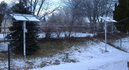
The interferometer that I am presently using has two small broadside array antennas. One antenna consists of 3 full-wave dipoles over a reflector, and the other antenna has 4 full-wave dipoles over a reflector. The two antennas of my interferometer are shown in Figure 3.
The antennas are about 7.5 meters or about 10 wavelengths apart. The baseline distance, declination and wavelength, determine the frequency of the cosine waveform or interferogram. With a wavelength of 0.75 meters (400 MHz), a source at zero declination (on the Equator) will produce a frequency of about 10 cycles per radian of source travel across the sky. The total beam-width of my antennas is about one radian (from null to null), so the interferograms that I get from sources at or near the Equator have a total of about 10 cycles.
Figure 4 shows an example plot of the output signal from my present radio interferometer. The plot shows interferograms from Taurus A (M1), Virgo A (M87) and the Sun. The antenna beams were set to a declination of 22 degrees to be centered on Taurus A. Virgo A at a declination of about 12 degrees is still well within the antenna beam, so it also appears on the plot. The sun, which normally produces a much greater response, was at a declination of about -21 degrees, so it was not even in the main antenna beam. Nevertheless, it produced the largest response of the three objects seen in the plot!
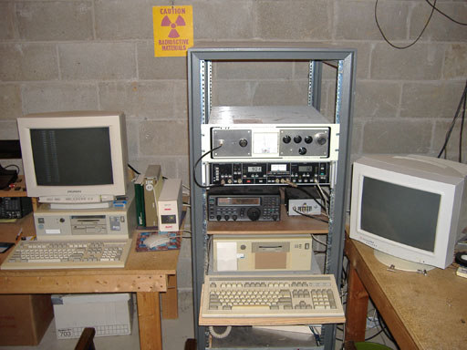
The indoor equipment used in my radio interferometer is shown in Figure 5. There are two computers, one for recording data and the other one for program development while recording data. Within the rack, the upper unit contains RF and back-end processing hardware. This equipment is home made. It consists of RF amplifiers, a phase switch, IF amplifiers, a square law detector, DC amplifiers and a low pass filter. I am using a phase switched interferometer with square law detection to implement the multiplying function of the interferometer described earlier. The signal from one of the antennas is switched in phase by 180 degrees periodically, and the detected signal is also synchronously phase switched to recover only the desired output product term from the square law detector. The synchronous detection is performed by a lock-in amplifier, which is located below the home made equipment chassis as seen in the figure. The output of the lock-in amplifier is sent to an A/D converter in the computer for data recording. An ICOM R8500 receiver is used for converting the 400 MHz incoming RF signal to a 10.7 MHz IF signal. The receiver is located below the lock-in amplifier. The small gray box to the right of the receiver is the phase switch driver. Either computer shown in the figure can be used for data recording or program development. The computer programs are run under the DOS operating system. This allows complete control of computer resources during data recording.
My future plans for this radio interferometer include developing antenna rotators for both antennas so that a source can be tracked over an 8 to 10 hour data collection period. This will provide the long interferograms needed for producing images by aperture synthesis. In the past, I have done aperture synthesis using small fixed dipole antennas that had very broad beams. The dipole antennas allowed collection of interferogram data over about 8 hours, and produced reasonable images, but the sensitivity of the system was severely limited by the small antennas. The solution to this problem is to use higher gain antennas with smaller beam-width, and track the source by keeping the antenna beams centered on the source. By installing rotators on the present larger antennas, I hope to produce images of weaker sources than the images I obtained previously with the small fixed dipole antennas.