
This is the second part of a two part article. If you haven’t done so already, read “Shooting M42: Part 1, An Introduction to Digital Deep-Sky Photography.”
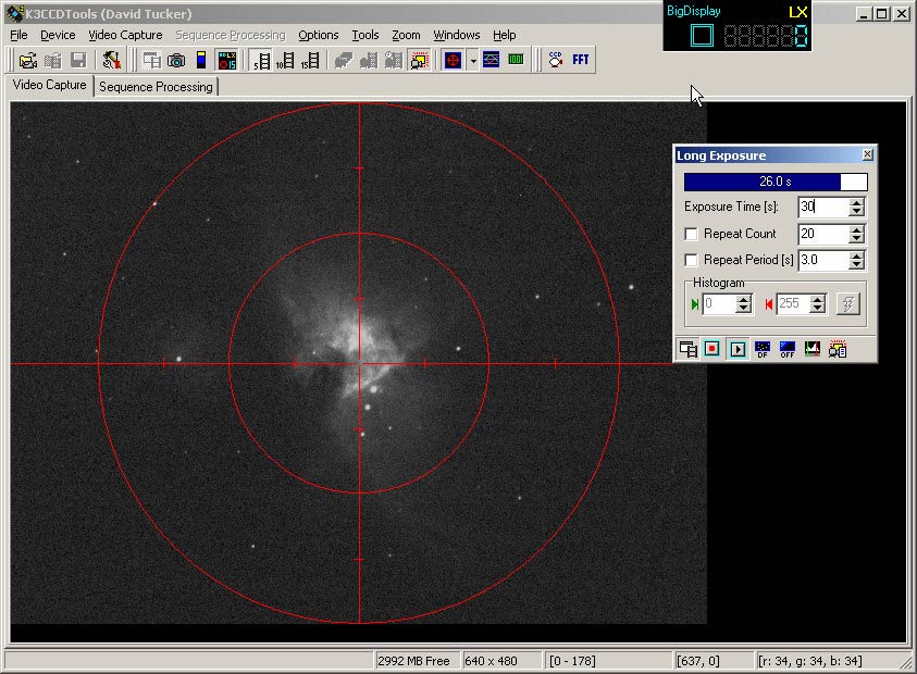
I do my image acquisition and most of my image processing using a program called K3CCD (from http://www.pk3.org/ ), written by Peter Katreniak. It’s reliable, easy to use, and I got a free copy with my camera. The software basically has two modes, called “Video Capture” and “Sequence Processing.” “Video Capture” mode is used for controlling the camera and saving images taken onto an avi file (basically a digital movie), and that’s the topic of this section. This is a typical screen shot while taking a series of long exposure images:
The “Long Exposure” Dialog allows me to enter the desired exposure length, number of frames to be taken. The program continuously updates the screen as images are “acquired” from the camera, and begins saving images to an AVI file as soon as the “record” button is clicked. Not shown is the “Amp Gain” control (accessed through “Device” on the main menu bar) which controls the gain on the cameras internal amplifier, which also can have a critical impact on the final image (discussed in the next section).
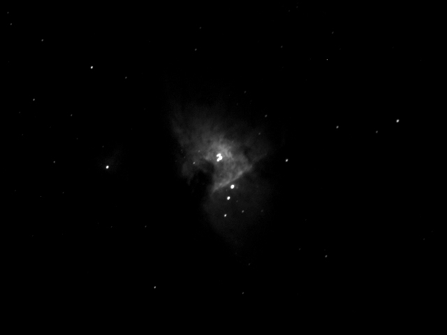
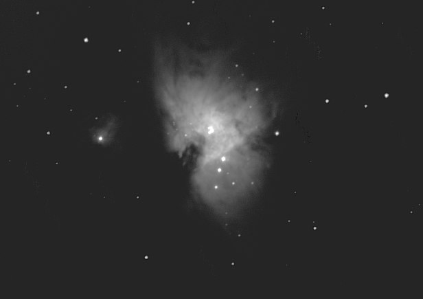
You may be wondering why I normally take long sequences of frames, rather then just one. Here is a single frame of M42, shown in its original form on the left, and “Gamma Adjusted” on the right to bring out dimmer pixels (“Gamma adjustment” is available in most photo-editing programs.) Here I adjusted “Gamma” from its default value of 1.0 up to 2.5:
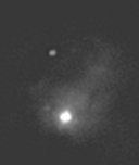
Here is a detail of the image on the right:
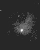
Not that great, is it? What were seeing here is mainly something referred to as “Quantum Noise.” The rules of physics dictate there will always be inherent inaccuracies when measuring subatomic particles like photons (the fundamental particles of light), but this inaccuracy drops as the quantity if photons measured increases. The most obvious way to increase the number of photons counted is to lengthen the exposure time, but there are limits here: No Equatorial Platform tracks perfectly (unless some sort of guiding setup is used), brighter features may saturate (overexpose), and then there’s that infernal “Dark Noise.” Infrared photons emitted by warm surfaces in the camera slowly clouding the image (remember, the camera is sensitive to IR as well as visible light—this problem can be partially dealt with by subtracting a “Dark Frame” taken with the lens cap on from the raw image, but I did not have to use this technique for this image, so I’m not going to go into it).
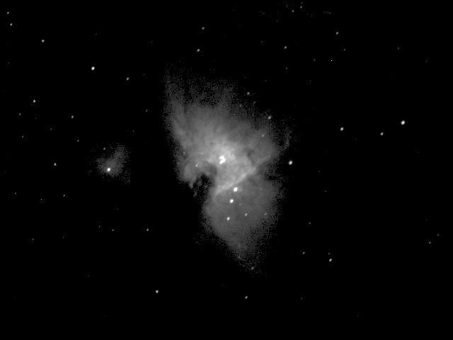
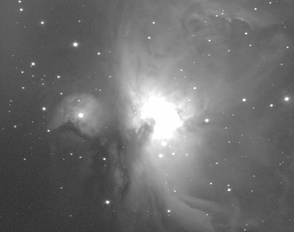
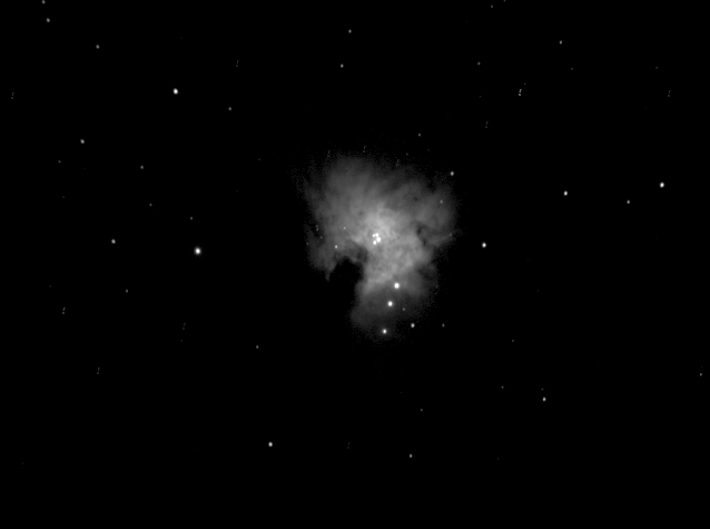
Digital technology offers us another option: we can take large numbers of moderate length frames (say, 30 seconds), and then have our Astro-Imaging software (K3CCD in this case) “Stack and Align” the images, then add corresponding pixels values on all of the frames together to give (say) a virtual one hour exposure. The alignment part of the process usually consists in have the user select a distinctive feature that appears in all of the frames (usually a star), the software will then automatically shift each image slightly (if necessary) to make up for minor equatorial tracking errors. I ended up taking around 180 odd 30 second exposures for this particular image, and this is the result (gamma adjusted):
Beautiful! Again, here is a detail:
It’s worth noting that by taking shorter sub frames we reduce the required polar tracking accuracy somewhat, but your not going to get a good picture if the object actually drifts out of the frame as you “film” it!
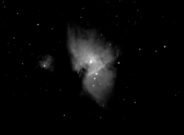
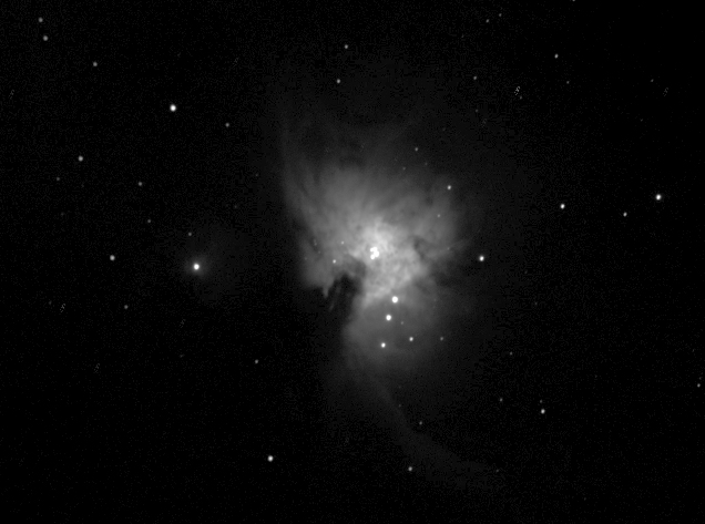
Finally, notice that my 180-frame image still has large area of black background, although in reality the whole region in suffused in dim nebulosity. To “fill in” the background, I either need to further extend exposure time/frame count, or increase the gain of the camera’s internal amplifier. I chose the later alternative, and cranked the gain up to 40% for a second run of images (in the first set the gain was set to zero). Here is the result:
Wow! here’s all the dim nebulosity missing from the first image, but the bright trapezium area is completely overexposed. But that’s ok, because I can use photo editing software (specifically, Registar) to paste the trapezium region from the first image onto the background of the second (I’ll get back to that).
Ideally the individual sub frames should be exposed for as long as possible (several minutes or more) when imaging really dim objects, but it’s often possible to get very good results using large “stacks” of 20 to 60 second frames. If frames are too short, there may be no image at all in darker parts of the image. To some extent we can correct this by increasing amp gain (as I did here), but that can significantly increase noise, especially as gain goes over about 50%. I often get everything set up, then take some test shots to find the largest practical sub frame length before I start to get star trailing due to tracking issues.
I stated earlier that we basically take color images through monochrome cameras by taking separate exposures (or “Stacks” of exposures) through Red, Green and Blue filters, then combine them using the “RGB Combine” functionality provided by most photo processing programs. But we can actually do better then this. By placing a color filter in front of the camera we are limiting the amount of light hitting the camera (e.g., a Red filter will block Blue and Green light), so the image will never be quite as good as a black-and-white image (unless the subject is particularly bright, like Jupiter maybe). So we introduce a fourth step into the process in which we combine the RGB image obtained by the RGB combine operation with a long exposure black-and-white image, called the “Luminance” image. This combine operation can be done using standard photo editing programs, like Photoshop or JASC Paintshop, by bring in the RGB image as one “layer” of a single image and the monochrome image as another, manually aligning them, and then merging the layers specifying “color” as the blend mode for the RGB image and “Luminance” for the monochrome. Typically I take many more monochrome frames the color frames, and almost all image processing (sharpening, etc.) is done to the luminance frame only before combining.
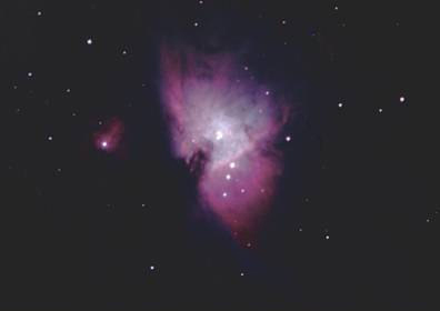
First I built an image of the bright core region, shooting about 150 30 second frames of “Luminance” (monochrome) data, then about 15 frames each through Red, Green, and Blue filters. From these I built four separate images representing the nebula in Red, Blue, Green and White light, doing the sub frame stacking in K3CCD.
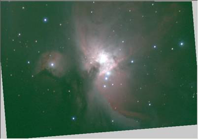
I then used “Registar” to combine the Red, Green, and Blue images into an RGB image, then finally used JASC Paintshop to merge in the Luminance data. This gave me the image below, on the left side.
Then, I did the whole thing all over again, this time with the Amp gain set at 40% to get the image below on the right. Finally I used “Registar” again to combine these two, to get the final image at the top of the article.
This is by far the most elaborate image I have ever taken—most of my images are monochrome, and I have never tried to combine images taken at multiple amplifier gain levels/exposure times before (and frankly, it will be a while before I do again!)
You can get more information on K3CCD from Peter Katreniak’s site http://www.pk3.org/Astro/index.htm , in particular see Carsten Arnholm’s tutorial at http://arnholm.org/astro/software/K3CCDTools/tut1/ (also available in Spanish!). There are too many good sources of imaging information on the web to possibly list, but one I particularly like the new Yahoo Small-Aperture-CCD group at http://groups.yahoo.com/group/small_aperture_ccd/?yguid=205602942 .
As far as books go, Ron Wodaski’s “The New CCD Astronomy” is about as close as you’ll come to a CCD imaging bible, and much of the technical information in this article came from that book. Or send an e-mail, maybe I’ll base my next newsletter article on the questions I get about this one.
My future plans include imaging some objects that don’t require recording and combining 6 separate stacks of images, getting some sleep, and seeing if I can run a coffeewarmer off the batterypack for my mounting.