


To apply system (2) to cross-sectional data, I assume that the
realization of system (1) in each district begins at small, random
displacements from 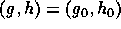 and
 . Each realization then runs for a random time
period with positive mean and finite variance. The precise form of the random
elements is not important, but it is convenient to assume that the random
elements are independently and identically distributed across districts. The
result is a data set consisting of the points at which the realizations
terminated.
Given only cross-sectional data, the equations of (2) have to be
simplified to eliminate parameters that are not uniquely identifiable with
such data. Parameters  ,
 and
 are not distinctly
defined: replacing with
 , with
 and with
 leaves
(2) unchanged. Further, for any choice of
 there is a
value of that leaves
 invariant. I normalize by
setting
 and collapsing into a single
parameter .
The next step is to build in transformations to adjust for the coordinate
system used to measure the observations  and
 . I
translate the observations to the origin using
 and
 where
 and
 are parameters with
values to be determined. I also allow the form of the periodic orbits (the
limit cycles of system (2)) to be elliptical rather than exactly
circular. As Figure 2 illustrates, ellipses ought to be better
approximations to the form of the orbits than circles would be. In system
(2) the appropriate change is to replace
 with
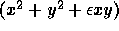 where
 is a parameter valued in the range
 .
To produce a statistical model I replace the time derivatives dx/dt and
dy/dt of system (2) with random variables  and
 , which
I assume to be bivariate normal with expectations
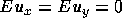 and
covariance matrix
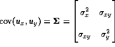 . I
assume that and are independently and identically distributed
across observations. The distributional assumption is justified by the fact
that the elliptical orbits are symmetric, and we expect observations to be
randomly distributed on orbits near the equilibrium. For observed data
and we now have the bivariate model
where , . Unknown parameters
are  ,
 , , , , and
 . Model (4) may be construed as specifying a
nonlinear covariance structure.
The bivariate model (4) illustrates the basic method of changing
time derivatives into random variables, but we should not expect a bivariate
specification to be sufficient to represent the dynamics of system
(1) near and the Cournot-Nash
equilibrium point . By the robustness of system
(2), we can reasonably treat the dynamics as two-dimensional. But
to represent system (2) in terms of the variables of system
(1) it is necessary to embed system (2) in a space of
dimension greater than two. Because system (2) is valid only in a
neighborhood of the equilibrium point, it is reasonable to consider the data
for which system (2) is relevant as confined to a compact set that
includes 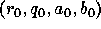 . Treating that set as a compact manifold in
which the flows of system (1) are occurring, we can then use the
Whitney embedding theorem (Hirsch 1976, 23-27) to conclude that a
four-dimensional model is necessary and sufficient to represent system
(2).
Indeed, we have direct evidence from system (1) that two-dimensional models will fail to recover the dynamics. In Figure 2, in the projection into the plane ``contributions to the challenger'' by ``probability that the incumbent wins,'' the flow of system (1) appears to cross itself. The resulting figure `8' pattern is fundamentally unlike the circular pattern of system (2)--a figure `8' cannot be smoothly mapped into a circle. Moreover, by the fundamental uniqueness theorems for differential equations, a flow that crosses itself is impossible (Hirsch and Smale 1974, 161-176). Therefore, even if system (1) were correct, a two-dimensional analysis of the relationship between challenger finances and votes would fail to confirm the dynamics of system (2), leading to the rejection of system (1). But the apparent failure of the model would be an artifact of the chosen pair of variables.
To do a four-dimensional analysis I extend model (4) to define
model (3), which in four equations combines the six models of form
(4) that can be constructed between pairs of the four observed
variables. The log-likelihood, for n observations, is  . To identify
the model I set
 , where k=28 is the number of parameters in model
(3). Doing so reduces the log-likelihood to
 .
