STATS 413: Lecture 25
-
Modeling probabilities
-
Maximum likelihood
-
Logistic regression
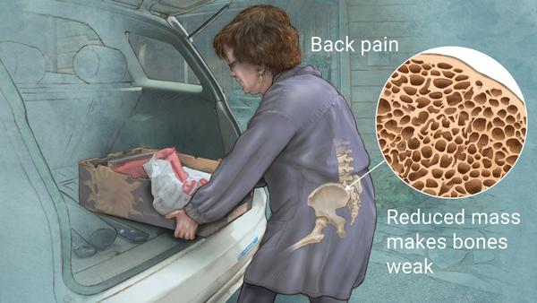
Diagnosing Osteoporosis
Osteoporosis is a bone disease leading to brittle bones.
-
Bones lose calcium.
-
Older women are more likely to have it than other demographics.
-
Lack of heavy lifting is a risk factor.
-
It is more prevalent in underweight people than overweight people.
Diagnosing Osteoporosis
Imagine a patient, an older woman, comes into the medical office.
-
X-ray is typically definitive.
-
Of course, X-ray is also expensive.
-
If the woman has a low risk for osteoporosis, maybe it is not worth it.
Let's run a simplified cost analysis.
Simplified Decision Process
Two possible states:
-
Patient has osteoporosis or does not have osteoporosis.
Two actions:
-
Send for X-ray or not.
Imagine the following values for the net cost of a given action:
| No X-ray | Yes X-ray | $P(\cdot)$ | |
|---|---|---|---|
| Okay | 0 | $400 | $1-p$ |
| Osteo | $3600 | 0 | $p$ |
| Expected Value | $3600$p$ | $400$(1-p)$ |
Rule: send for X-ray if $400(1-p)\leq 3600p \Rightarrow \mathbf{p \geq 1/10}$.
Osteoporosis Data
Our data set contains $n=864$ patients and 6 covariates.
-
Response: whether the individual has osteoporosis.
-
Covariates: various risk factors.
-
The covariates include:
-
Weight
-
Age
-
Height
-
Years taking estrogen supplement
-
Calcium supplement?
-
Recent bone fracture?
-
Osteoporosis Data
We randomly split into a training set and a test set. We will now look at the training set of size $n_{\text{train}} = 604$.
Modeling Binary Data
For the moment, suppose we only had access to whether or not an individual in the training set has osteoporosis, with no other information.
Suppose our data set could be modeled as $n$ i.i.d. random variables.
-
What random variable would we use to model whether or not the $i$-th individual has osteoporosis?
-
Do we know the parameter that governs this random variable?
-
How would we estimate it based on our training set?
-
How would we conduct inference for it?
Let's Construct a Baseline Model
From the training data:
-
228 individuals have osteoporosis.
-
376 individuals do not have osteoporosis.
For now, we will ignore the cost analysis and focus on correctly classifying whether or not an individual has osteoporosis.
-
If I have no other information beyond the fact that the person is from the population of interest, what should I predict in order to maximize accuracy, the percentage of correct classifications?
A Baseline Model
Baseline model: always predict that a person does not have osteoporosis.
-
Correct on all 165 individuals in the test set without osteoporosis.
-
Incorrect on 95 individuals in the test set with osteoporosis.
Obtains 63% accuracy in the test set with no real work.
-
But we have all sorts of other information.
-
We would certainly hope to do better in predicting osteoporosis based on other covariates.
A Baseline X-Ray Decision
Let's return to the cost analysis. The decision rule was to send for X-ray if $400(1-p)\leq 3600p \Rightarrow \mathbf{p \geq 1/10}$.
From my training set, $\hat{p} = 0.39$.
-
If I have no other information for each individual, what should my decision be? Send everyone to get an X-ray.
In the test set, 165 out of 260 individuals do not have osteoporosis.
-
Average cost of $(165/260)400 = 253.84$.
Again, might we be able to use covariate information to reduce costs?
Linear Regression with 0-1 Responses
Our first instinct might be to fit a regression model
\[ \hat{y}_i = \hat{\beta}_0 + \hat{\beta}_1x_{i1} + \cdots + \hat{\beta}_p x_{ip} \]Multiple regression attempts to model the conditional expectation of $y_i$ given $x_i$.
If linearity held, then
\[ E(y_i \mid x_i) = \beta_0 + \beta_1x_{i1} + \cdots + \beta_p x_{ip} \]What does the expectation of a binary variable equal?
\begin{align*} E(y_i \mid x_i) &= 1 \times P(y_i=1 \mid x_i) + 0 \times P(y_i=0 \mid x_i) \\ &= P(y_i=1 \mid x_i) \end{align*}Linear Regression with 0-1 Responses
In the binary-response setting, the multiple regression model would say that
\[ p(x_i) = P(Y_i=1 \mid x_i) = \beta_0 + \beta_1x_{i1} + \cdots + \beta_p x_{ip} \]That is, the probability of success is linear in the covariates.
The regression line returned by R would then be providing estimates for the probability of
success:
To visualize, let's consider a simple regression example with a binary response.
Osteoporosis and Weight
The y variable here is an indicator of whether or not an individual in the data set has
osteoporosis, while x is the individual's weight.

The line, believe it or not, is the line of best fit.
Other Issues
Even if the probabilities were linear in the covariates, there are other issues when using linear regression to fit binary outcomes. The stronger linear model cannot hold.
-
$\varepsilon_i$ terms cannot be normally distributed if the outcome is binary. That would imply continuous responses.
Other Issues
If $y$ is Bernoulli with probability of success given $x$ equal to $p(x)$, then
\[ \operatorname{var}(y \mid x) = p(x)\{1-p(x)\} \]-
Homoskedasticity also cannot hold. The variance of the responses varies with $x_i$.
While these issues could be remediated with HC standard errors and with the bootstrap, given the fundamental issues with linearity when predicting probabilities, we take a different approach.
The Logit Link Function
Directly fitting a linear model to binary data fails to account for the constraint that $0\leq p(x)\leq 1$.
-
Instead of fitting a linear function for $p(x)$, we can fit a linear function of some transformation of $p(x)$ that is unbounded.
-
This is called finding a link function.
For regression with binary responses, by far the most common choice is the logit link:
\[ \operatorname{logit}(p(x)) = \log\left(\frac{p(x)}{1-p(x)}\right) \]$\operatorname{logit}(p(x))$ is also known as the log-odds, since $p(x)/(1-p(x))$ is the odds of observing a 1 given $x$.
Linear on the Logit Scale
We now imagine that a linear model holds on the logit scale:
\[ \log\left(\frac{p(x_i)}{1-p(x_i)}\right) = \beta_0 + \beta_1x_{i1} + \cdots + \beta_p x_{ip} \]Solving for $p(x_i)$ yields
\[ \textstyle p(x_i) = \frac{\exp\{\beta_0 + \beta_1x_{i1} + \cdots + \beta_p x_{ip}\}} {1+\exp\{\beta_0 + \beta_1x_{i1} + \cdots + \beta_p x_{ip}\}} \]-
$\beta_j$ are unknown parameters of the model, governing the true probability of a 1 given $x$.
-
Given our data set, we seek to estimate $\beta_j$.
First: the Logistic Function
\[ \operatorname{logistic}(\theta) = \frac{\exp\{\theta\}}{1+\exp\{\theta\}} \]
First: the Logistic Function
Properties:
-
$0 < \operatorname{logistic}(\theta) < 1$
-
$\operatorname{logistic}(0)=\frac{1}{2}$
-
$\operatorname{logistic}(\theta)$ is an increasing function of $\theta$
Now let $\theta = \beta_0 + \beta_1x_1 + \cdots + \beta_p x_p$.
-
If $\beta_j > 0$, then the function is increasing in $x_j$.
-
If $\beta_j < 0$, then the function is decreasing in $x_j$.
Logistic Regression
We will use the observed data to estimate the parameters $\beta_0,\dots,\beta_p$. That is, we will use data to estimate
\[ \textstyle p(x) = \frac{\exp\{\beta_0 + \beta_1x_{i1} + \cdots + \beta_p x_{ip}\}} {1+\exp\{\beta_0 + \beta_1x_{i1} + \cdots + \beta_p x_{ip}\}} \]by means of
\[ \textstyle \hat{p}(x) = \frac{\exp\{\hat{\beta}_0 + \hat{\beta}_1x_{i1} + \cdots + \hat{\beta}_p x_{ip}\}} {1+\exp\{\hat{\beta}_0 + \hat{\beta}_1x_{i1} + \cdots + \hat{\beta}_p x_{ip}\}} \]The process of fitting the function $\hat{p}(x)$ is known as logistic regression.
Predicting Osteoporosis
glm(Osteo ~ Weight, family = "binomial", data = train)

Coefficients:
(Intercept)       Weight
4.52637 -0.03183The Prediction Function
Here is a plot of the estimated $\hat{p}(x)$. Again, points are jittered to avoid overplotting.

Finding the Equation
How did R come up with this equation?
-
In linear regression,
Rfinds the line that minimizes the in-sample SSE. -
With binary data, that strategy does not respect the fact that we are predicting probabilities.
Instead, R comes up with this equation through maximum likelihood estimation.
First: the Distribution Function
Suppose I knew the values of $\beta_0,\beta_1,\dots,\beta_p$.
At any point $x_i = (1,x_{i1},\dots,x_{ip})^\top$, what is the probability of observing a one given $x_i$? What about a zero?
\[ \textstyle P(y_i=1 \mid x_i) = \frac{\exp\{x_i^\top\beta\}}{1+\exp\{x_i^\top\beta\}}, \qquad P(y_i=0 \mid x_i) = \frac{1}{1+\exp\{x_i^\top\beta\}} \]I can write this concisely as
\[ \textstyle p(y_i \mid x_i) = \left(\frac{\exp\{x_i^\top\beta\}}{1+\exp\{x_i^\top\beta\}}\right)^{y_i} \left(\frac{1}{1+\exp\{x_i^\top\beta\}}\right)^{1-y_i} \]Do you see why? Evaluate by setting $y_i=1$ and $y_i=0$.
Second: The Joint Probability
In my data set, I have $n$ pairs $(x_1,y_1),\dots,(x_n,y_n)$. We assume independence between observations.
Given $x_1,x_2,\dots,x_n$, what is the probability of observing $y_1$ and $y_2$ and $\cdots$ and $y_n$?
\[ p(y_1 \cap y_2 \cap \cdots \cap y_n \mid x_1,\dots,x_n) = \prod_{i=1}^n p(y_i \mid x_i) \] \begin{align*} &p(y_1 \cap y_2 \cap \cdots \cap y_n \mid x_1,\dots,x_n) = \\ &\quad\prod_{i=1}^n \left(\frac{\exp\{x_i^\top\beta\}}{1+\exp\{x_i^\top\beta\}}\right)^{y_i} \left(\frac{1}{1+\exp\{x_i^\top\beta\}}\right)^{1-y_i} \end{align*}Finally: The Likelihood Function
Plugging in the values of $y_i$ and $x_i$ from my data gives
\[ \textstyle P(y \mid x) = \prod_{i=1}^n \left(\frac{\exp\{x_i^\top\beta\}}{1+\exp\{x_i^\top\beta\}}\right)^{y_i} \left(\frac{1}{1+\exp\{x_i^\top\beta\}}\right)^{1-y_i} \]I know $\{y_i\}$ and $\{x_i\}$ from my data, but $\beta_0,\dots,\beta_p$ are unknown.
What values for $\beta = (\beta_0,\dots,\beta_p)^\top$ maximize the likelihood of observing the data?
\[ \textstyle \hat{\beta} = \underset{\beta}{\operatorname{arg\,max}} \; \prod_{i=1}^n \left(\frac{\exp\{x_i^\top\beta\}}{1+\exp\{x_i^\top\beta\}}\right)^{y_i} \left(\frac{1}{1+\exp\{x_i^\top\beta\}}\right)^{1-y_i} \]There is no closed-form solution, but we can solve it numerically.
Finally: The Likelihood Function
The maximizers, often called the MLEs for maximum likelihood estimates, are
\[ \hat{\beta} = (\hat{\beta}_0,\hat{\beta}_1,\dots,\hat{\beta}_p)^\top \]Familiar MLEs
Many familiar estimators can be motivated as maximum likelihood estimators under specific distributional assumptions.
-
If $y_1,\dots,y_n$ are i.i.d. Bernoulli with unknown probability of success $p$, then $\hat{p}$, the fraction of ones in the data, is the MLE.
-
If $y_1,\dots,y_n$ are i.i.d. Normal with unknown mean $\mu$ and unknown standard deviation $\sigma$, then the MLE for $\mu$ is $\bar{y}$.
-
Under the stronger linear model,
with $\varepsilon_i$ i.i.d. with mean zero and standard deviation $\sigma_\varepsilon$, the MLEs for $(\beta_0,\beta_1,\dots,\beta_p)$ are the OLS coefficients,
\[ (\hat{\beta}_0,\hat{\beta}_1,\dots,\hat{\beta}_p) = (X^\top X)^{-1}X^\top y \]Where'd the Coefficients Come From?
Define $L(\beta \mid y, x)$ as
\[ \textstyle L(\beta \mid y, x) = \prod_{i=1}^n \left(\frac{\exp\{\beta_0+\sum_{j=1}^p\beta_jx_{ij}\}} {1+\exp\{\beta_0+\sum_{j=1}^p\beta_jx_{ij}\}}\right)^{y_i} \left(\frac{1}{1+\exp\{\beta_0+\sum_{j=1}^p\beta_jx_{ij}\}}\right)^{1-y_i} \]We find the coefficients $\{\hat{\beta}_j\}$ through the following optimization problem:
\[\textstyle \argmax_\beta\; L(\beta \mid y, x) \]Or, equivalently due to monotonicity of the logarithm,
\[\textstyle \argmin_\beta\; -\log\left(L(\beta \mid y, x)\right) \]In practice, most maximum likelihood estimators are actually found by minimizing the negative log likelihood.
Log Loss
Define $p_\beta(x_i)$ as what the probability would be given $x_i$ for a fixed value of $\beta$:
\[ \textstyle p_\beta(x_i) = \frac{\exp\{\beta_0+\sum_{j=1}^p\beta_jx_{ij}\}} {1+\exp\{\beta_0+\sum_{j=1}^p\beta_jx_{ij}\}} \]Taking the negative of the log likelihood,
\begin{align*} &-\log\left(L(\beta \mid y, x)\right) \\ &\textstyle\quad=\sum_{i=1}^n \{-y_i\log(p_\beta(x_i))-(1-y_i)\log(1-p_\beta(x_i))\} \end{align*}The log loss for a predicted probability $\theta_i$ and observed outcome $y_i$ is
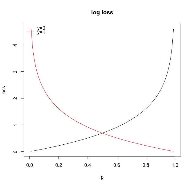
\[ -y_i\log(\theta_i) - (1-y_i)\log(1-\theta_i) \]Log Loss
Useful to break this down into cases:
\[ \begin{cases} -\log(\theta_i) & y_i = 1\\ -\log(1-\theta_i) & y_i = 0 \end{cases} \]-
When the outcome is one, loss is smallest when $\theta_i = 1$ and tends to infinity as $\theta_i$ goes to zero.
-
When the outcome is zero, loss is smallest when $\theta_i = 0$ and tends to infinity as $\theta_i$ goes to one.
Log Loss
Linear vs Logistic Regression
Linear regression and logistic regression both choose $\hat{\beta}$ by minimizing the sum of losses, but they differ in their choice of loss function.
-
Linear regression minimizes the sum of squared error losses.
-
Logistic regression minimizes the sum of log losses.
Multiple Logistic Regression
Here is the logistic regression fit for our osteoporosis data using all available covariates.
glm(Osteo ~ ., family = "binomial", data = train)
Coefficients:
   (Intercept)          Weight             Age          Height
       2.29400        -0.03068         0.06857        -0.03749
Years.estrogen         Calcium        Fracture
-0.02088 -0.04248 0.96610Again, All Else Equal...
Our interpretation for any of the estimated slope coefficients $\hat{\beta}_j$, $j=1,\dots,p$, from logistic regression depends upon the other variables within the model.
Ceteris Paribus
All else equal, two individuals who differ in variable $x_j$ by 1 unit are estimated to differ in their log-odds of success by $\hat{\beta}_j$, or equivalently by an odds ratio of $\exp\{\hat{\beta}_j\}$.
Again, All Else Equal...
That is, $\hat{\beta}_j$ is the estimated difference in log-odds for two individuals who differ in covariate $x_j$ by 1 unit, but have the same values for all of the other predictor variables.
In Terms of Probabilities
Unfortunately, the model is not linear on the probability scale.
The resulting difference in predicted probability depends on the particular values of the covariates.
At the very least, we can interpret the sign.
-
Positive $\hat{\beta}_j \Rightarrow$ all else fixed, higher values of $x_j$ have higher predicted probability.
-
Negative $\hat{\beta}_j \Rightarrow$ all else fixed, higher values of $x_j$ have lower predicted probability.
Inference in Logistic Regression
The summary table from logistic regression looks very similar to that of linear regression.
Coefficients:
                Estimate Std. Error z value Pr(>|z|)
(Intercept)     2.294001   2.625111   0.874 0.382190
Weight         -0.030680   0.004189  -7.324 2.40e-13 ***
Age             0.068569   0.011672   5.874 4.24e-09 ***
Height         -0.037486   0.038888  -0.964 0.335066
Years.estrogen -0.020881   0.012125  -1.722 0.085050 .
Calcium        -0.042481   0.268710  -0.158 0.874384
Fracture        0.966103   0.265801   3.635 0.000278 ***
---
Signif. codes:  0 '***' 0.001 '**' 0.01 '*' 0.05 '.' 0.1 ' ' 1
Generalized Linear Models
Logistic regression and linear regression are two members of a broader class of models known as generalized linear models.
This class involves
-
Distributional assumption on the outcome variable
-
Link function: a transformation $g$ of $E(y \mid x)$ that is modeled as linear in $x$
Generalized Linear Models
Examples:
- Linear regression: normal distribution, identity link
- Logistic regression: Bernoulli distribution, logit link
- Poisson regression: Poisson distribution, log link
The function glm allows us to fit generalized linear models.