STATS 413: Lecture 24
-
Regularization
-
Ridge Regression
-
LASSO
Towards an Alternative Approach
We can write the objective function for best subsets as
\begin{align*} \sum_{i=1}^n \left(y_i - \left(\beta_0 + \sum_{j=1}^p \beta_j x_{ij}\right)\right)^2 + \lambda \sum_{j=1}^p |\beta_j|^0, \end{align*}where we define
\begin{align*} |\beta_j|^0 := \lim_{q \rightarrow 0^+} |\beta_j|^q &= \begin{cases} 0 & \beta_j = 0 \\ 1 & \text{otherwise.} \end{cases} \end{align*}Towards an Alternative Approach
Rather than thinking of greedy heuristics for best subset selection, such as forward stepwise or backward elimination, we could instead change the form of the complexity penalty:
\begin{align*} \sum_{i=1}^n \left(y_i - \left(\beta_0 + \sum_{j=1}^p \beta_j x_{ij}\right)\right)^2 + \lambda \sum_{j=1}^p |\beta_j|^q,\;\; q > 0 \end{align*}Contours of $|\beta_1|^q + |\beta_2|^q$
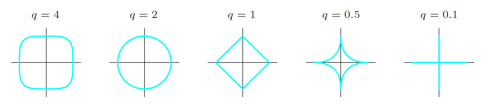
The figure shows contours of equal value satisfying $|\beta_1|^q + |\beta_2|^q = 1$.
-
As $q$ tends toward zero, the penalty behaves more like $|\beta_1|^0 + |\beta_2|^0$.
-
For $q \geq 1$, the corresponding regions are convex sets.
-
For $q > 1$, the boundaries are smooth as they intersect the axes.
Regularization
The following optimization problem is referred to as $\ell_q$-regularized regression for $q \geq 0$:
\begin{align*}\textstyle \underset{\beta}{\arg\min}\;\; \sum_{i=1}^n \left(y_i - \left(\beta_0 + \sum_{j=1}^p \beta_j x_{ij}\right)\right)^2 + \lambda \sum_{j=1}^p |\beta_j|^q. \end{align*}Importantly, for $q \geq 1$, the objective function is convex in $\beta$.
Regularization
-
Implication: it can be solved to optimality efficiently.
-
Rather than resorting to heuristics for best-subset selection, this changes the complexity penalty in a computationally tractable way.
-
As before, we do not penalize the intercept, since it only finds the right vertical level for the fitted line.
Most common in practice are $\ell_1$- and $\ell_2$-regularized regression, better known as LASSO and ridge regression.
Correcting a Deficiency
\begin{align*}\textstyle \underset{\beta}{\arg\min}\;\; \sum_{i=1}^n \left(y_i - \left(\beta_0 + \sum_{j=1}^p \beta_j x_{ij}\right)\right)^2 + \lambda \sum_{j=1}^p |\beta_j|^q \end{align*}For this to be a sensible criterion, we need to standardize, or $z$-score, the predictor variables $x_1,\dots,x_p$.
-
Reason: slope coefficients $\beta_j$ depend on the units of $x_j$.
-
If $x_j$ were temperature, changing from Fahrenheit to Celsius would change the magnitude of $\beta_j$.
-
Without adjustment, the criterion would penalize a predictor differently depending on the units used.
-
It would also create different degrees of penalization across predictor variables measured in different units.
Standardized Predictors
When running regularized regression with $q > 0$, we perform a $z$-score transformation on each predictor variable:
\begin{align*} z(x_{ij}) = \frac{x_{ij} - \bar{x}_j}{\operatorname{sd}(x_j)}, \end{align*}where $\bar{x}_j$ and $\operatorname{sd}(x_j)$ are the sample mean and standard deviation for the $j$th predictor.
Standardized Predictors
-
This is also called standardizing the predictor variables.
-
$z(x_{ij})$ is not affected by changes in units.
-
All predictors are placed on the same scale: standard deviations above or below the mean.
Moving forward, assume the predictors have been standardized so that $\bar{x}_j = 0$ and $\operatorname{sd}(x_j) = 1$.
Ridge Regression
We begin with ridge regression, corresponding to $q = 2$. It replaces ordinary least squares with
\begin{align*}\textstyle \underset{\beta}{\arg\min}\;\; \sum_{i=1}^n \left(y_i - \left(\beta_0 + \sum_{j=1}^p \beta_j x_{ij}\right)\right)^2 + \lambda \sum_{j=1}^p |\beta_j|^2. \end{align*}-
$\lambda = 0$: ordinary least squares with all variables.
-
$\lambda \rightarrow \infty$: the slope coefficients $\hat{\beta}_j$ shrink toward zero.
-
For this reason, regularized regression methods with $q > 0$ are often called shrinkage methods.
Ridge regression is particularly useful when $X^\top X$ is not invertible, or when strong multicollinearity is present.
Ridge Regression
Let $X$ be an $n \times p$ design matrix with the intercept removed, so the first column is $x_1$, the second is $x_2$, and so on. Assume the predictors have already been standardized.
For a given $\lambda$, the ridge regression problem yields slope coefficients $(\hat{\beta}_{\lambda 0}^R, \hat{\beta}_{\lambda}^R)^\top$ of the form
\begin{align*} \hat{\beta}_{\lambda 0}^R &= \bar{y} \\ \hat{\beta}_{\lambda}^R &= (X^\top X + \lambda I)^{-1} X^\top y, \end{align*}-
Even if $X^\top X$ is not invertible, $X^\top X + \lambda I$ will be.
-
In general, $(X^\top X + \lambda I)^{-1}$ is more stable than $(X^\top X)^{-1}$.
-
This is especially useful under multicollinearity.
Properties of Ridge Regression
Let's investigate the expectation and variance of the ridge coefficients.
Expectation and Variance of Ridge Regression
Suppose the weaker linear model holds, and let $\beta = (\beta_1,\dots,\beta_p)$.
\begin{align*} E(\hat{\beta}^R_\lambda) &= (X^\top X + \lambda I)^{-1} X^\top X \beta, \\ \operatorname{Var}(\hat{\beta}^R_\lambda) &= \sigma^2_\varepsilon (X^\top X + \lambda I)^{-1} X^\top X (X^\top X + \lambda I)^{-1} \end{align*}Properties of Ridge Regression
Implication:
-
Unless $\lambda = 0$, $\hat{\beta}^R_\lambda$ is a biased estimator of $\beta$.
-
For $\lambda > 0$, its variance is always smaller than that of the OLS solution.
-
Ridge regression sacrifices unbiasedness in exchange for stability by trading increased bias for reduced variance.
The Bias-Variance Tradeoff
Recall that the Gauss-Markov theorem says that among linear, unbiased estimators, $\hat{\beta}_{OLS}$ has the smallest variance under the weaker linear model.
-
Corollary: among unbiased, linear estimators, $\hat{\beta}_{OLS}$ has the smallest prediction error under homoskedasticity and linearity.
The Bias-Variance Tradeoff
When forming predictions for $y^*$ with covariate $\tilde{x}$, we have
\begin{align*} \text{Prediction Error} = \text{Irreducible Error} + \text{Squared Bias} + \text{Variance} \end{align*}Gauss-Markov does not rule out the existence of biased estimators with better prediction error than $\hat{\beta}_{OLS}$.
-
Regularized regression methods try to exchange increased squared bias for reduced variance in a way that improves prediction error.
-
This is especially beneficial under multicollinearity, or when $n \approx p$.
Ridge Regression Bias-variance Tradeoff
-
Black: bias of ridge regression.
-
Green: variance of ridge regression.
-
Purple: prediction error.
-
Left: plotted as a function of $\lambda$. Right: plotted as a function of the relative magnitude of the ridge and OLS coefficients.
-
Increasing $\lambda$ increases bias but decreases variance.
Ridge Regression Bias-variance Tradeoff

Illustration: The Diabetes Dataset
Here is the impact of $\lambda$ on the ridge coefficient values when fit to the extended diabetes data set with $p = 64$.
-
Each line tracks a particular slope coefficient.
-
The paths are not monotone in $\lambda$ because multicollinearity is still present.
-
The coefficients do tend to zero as $\lambda \rightarrow \infty$.
-
They are never exactly zero for any finite $\lambda$.
Illustration: The Diabetes Dataset

Benefits and Limitations of Ridge Regression
Computationally, ridge regression is easy to fit.
-
It is no harder than ordinary least squares and comes with extra numerical stability.
With $\lambda$ chosen by cross-validation, it can improve out-of-sample performance relative to a model that includes all variables.
-
This reflects an effective bias-variance tradeoff.
Benefits and Limitations of Ridge Regression
The primary drawback is that ridge regression never actually sets a coefficient equal to zero.
-
The resulting prediction equation always depends on all $p$ coefficients.
-
It is not performing model selection in the sense of finding a subset of the predictor variables.
-
It can yield stable predictions for future observations, but the fitted equation still depends on every predictor.
LASSO Regression
LASSO regression replaces the $\ell_2$ penalty of ridge with an $\ell_1$ penalty on the magnitudes of the slope coefficients:
\begin{align*}\textstyle \underset{\beta}{\arg\min}\;\; \sum_{i=1}^n \left(y_i - \left(\beta_0 + \sum_{j=1}^p \beta_j x_{ij}\right)\right)^2 + \lambda \sum_{j=1}^p |\beta_j| \end{align*}-
LASSO stands for Least Absolute Shrinkage and Selection Operator.
-
As before, the predictors $x_{ij}$ are assumed to be standardized.
Properties of LASSO Solution
Unlike ridge regression, there is not generally a closed-form solution for the LASSO coefficient estimates.
-
The objective is still convex, so we can find the global optimum using convex optimization algorithms.
As with ridge regression:
-
The LASSO coefficients $\hat{\beta}^L_\lambda$ are biased estimates of $\beta$ for any $\lambda > 0$.
-
LASSO tries to trade increased bias for improved variance and stability to improve overall prediction error.
-
Cross-validation is essential for navigating this tradeoff.
LASSO and Variable Selection
Unlike ridge regression, LASSO can set slope coefficients exactly equal to zero, making the resulting prediction equation much more interpretable.

LASSO and Variable Selection
Why does LASSO perform variable selection, whereas ridge does not?
-
$|\beta_j|^2 = \beta_j^2$ is differentiable at $\beta_j = 0$.
-
$|\beta_j|$ is not differentiable at $\beta_j = 0$.
For more intuition, we can equivalently write LASSO and ridge in constrained form for $q = 1$ and $q = 2$, respectively:
\begin{align*} \underset{\beta}{\arg\min}\;\; &\textstyle\sum_{i=1}^n \left(y_i - \left(\beta_0 + \sum_{j=1}^p \beta_j x_{ij}\right)\right)^2 \\ \text{subject to}\;\; &\textstyle\sum_{j=1}^p |\beta_j|^q \leq C_\lambda \end{align*}For every $\lambda$ in the original formulation, there exists a value $C_\lambda$ such that the two problems return identical slope coefficients.
Constrained Optimization
The plot shows contours of equal $SSE$ in red, along with the constraint sets in blue for LASSO (left) and ridge (right).
-
The LASSO and ridge solutions occur at the first intersection between the contour lines and the constraint set.
-
Because the LASSO constraint set has sharp corners, the intersection can occur when a collection of coefficients equals zero.
Constrained Optimization
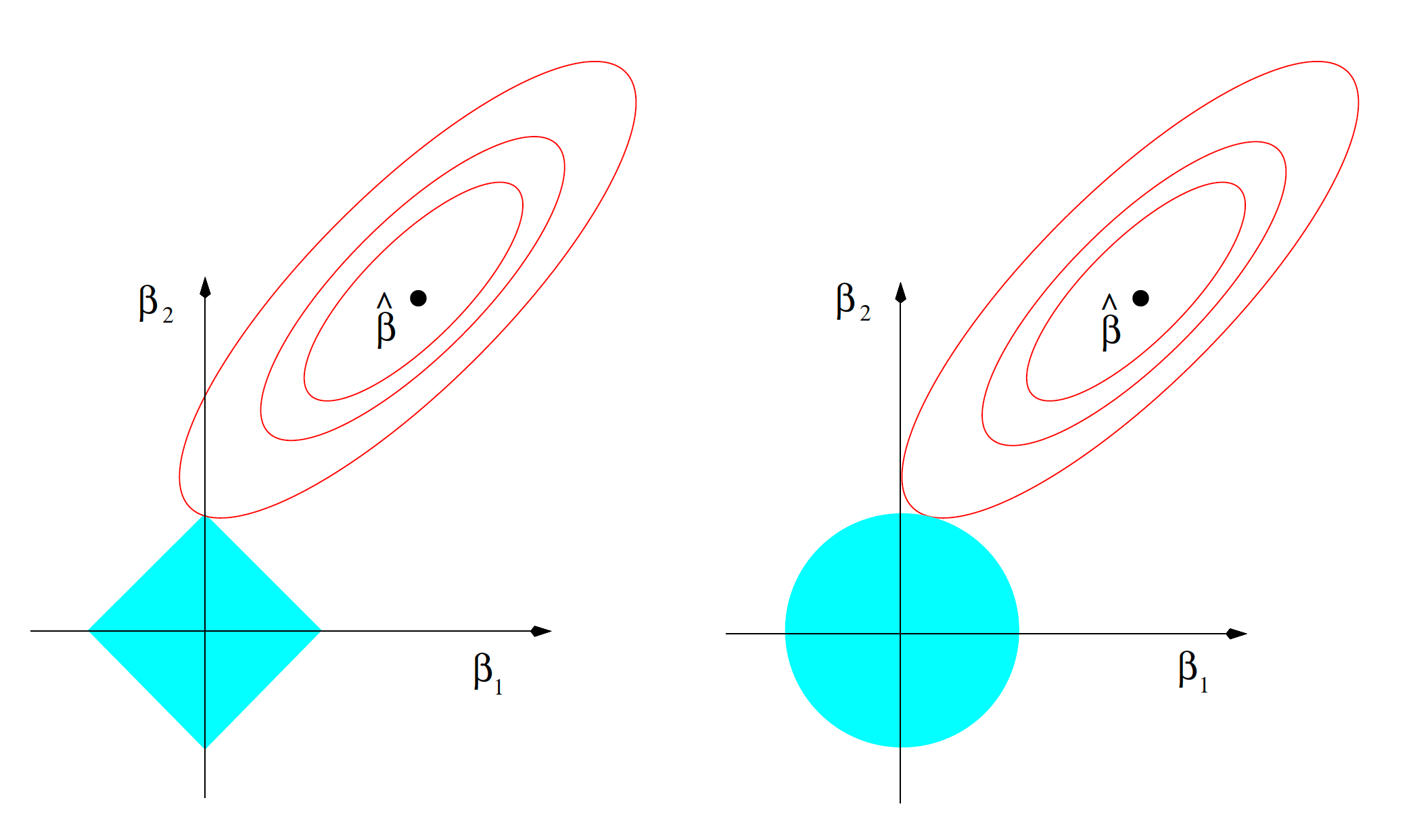
Illustration: The Diabetes Dataset
Here is the impact of $\lambda$ on the LASSO coefficient values when fit to the extended diabetes data set with $p = 64$.
-
The paths are not monotone in $\lambda$ because of multicollinearity.
-
The coefficients do tend to zero as $\lambda \rightarrow \infty$.
-
Coefficients can be set exactly equal to zero.
-
Beyond a certain $\lambda$, all coefficients are zero.
Illustration: The Diabetes Dataset

Extended Diabetes Regression Model
| Algorithm | Model Size ($m$) | $R^2$ | $OSR^2$ |
|---|---|---|---|
| Full Model | 64 | 0.631 | 0.340 |
| AIC, backward | 29 | 0.611 | 0.335 |
| BIC, backward | 13 | 0.585 | 0.358 |
| AIC, forward | 14 | 0.587 | 0.370 |
| BIC, forward | 5 | 0.537 | 0.416 |
Extended Diabetes Regression Model
| Algorithm | Model Size ($m$) | $R^2$ | $OSR^2$ |
|---|---|---|---|
| Cross-validated, forward | 8 | 0.561 | 0.463 |
| Cross-validated, backward | 14 | 0.585 | 0.358 |
| Ridge, Cross-validated | 64 | 0.585 | 0.426 |
| LASSO, Cross-validated | 16 | 0.562 | 0.444 |
-
Based on this assessment, we would still choose the forward-selection model with tuning chosen by cross-validation.
-
That will not be true for every data set. Sometimes ridge or LASSO will perform better, so the methods should be compared on a test set.
Regression in High Dimensions
When we introduced ordinary least squares, we required that $X^\top X$ was invertible.
-
This fails under perfect multicollinearity.
-
It also fails when $p \geq n$, meaning there are at least as many predictors as observations.
In some domains, it is common to have $p \gg n$.
-
So far, our data sets have had many more rows than columns.
-
Sometimes "big data" means many features: a large number of columns with a limited number of rows.
Regression in High Dimensions
A common assumption in these settings is that many of the coefficients $\beta_j$ are actually zero.
-
There may be many candidate predictors, but only a few are truly important.
-
This is known as a sparse regression context.
Genome Wide Association Studies
-
A classic example is genome wide association studies, or GWAS.
-
The objective is to discover whether any genes are associated with a given health condition.
-
$n$: number of individuals, which could be in the hundreds or thousands.
-
$x_j$: indicator of whether a particular gene is present.
-
$p$: hundreds of thousands of candidate genes.
In settings with $p \gg n$, ordinary least squares using all $p$ predictors falls short.
What Goes Wrong with OLS?
Consider the following system of equations:
\begin{align*} y_1 &= \hat{\beta}_0 + \hat{\beta}_1 x_{11} + \cdots + \hat{\beta}_p x_{1p} \\ y_2 &= \hat{\beta}_0 + \hat{\beta}_1 x_{21} + \cdots + \hat{\beta}_p x_{2p} \\ &\vdots \\ y_n &= \hat{\beta}_0 + \hat{\beta}_1 x_{n1} + \cdots + \hat{\beta}_p x_{np} \end{align*}If $p \geq n - 1$ and the rows of $X$ are linearly independent, we can perfectly fit the observed data and obtain in-sample $SSE = 0$.
What Goes Wrong with OLS?
-
If $p + 1 = n$, we can find a single value of $\hat{\beta}$ that perfectly reproduces the observed response vector.
-
If $p \geq n$, there are generally infinitely many values of $\hat{\beta}$ that perfectly reproduce the observed responses.
This is an extreme example of overfitting.
Regularization to the Rescue
In high-dimensional settings, LASSO has particular appeal:
\begin{align*}\textstyle \underset{\beta}{\arg\min}\;\; \sum_{i=1}^n \left(y_i - \left(\beta_0 + \sum_{j=1}^p \beta_j x_{ij}\right)\right)^2 + \lambda \sum_{j=1}^p |\beta_j| \end{align*}-
It remains computationally feasible even when $p$ is in the thousands or millions.
-
By penalizing complexity, it helps avoid overfitting.
-
Ridge would be less appealing here, even though it is still computationally feasible, because all covariates would retain nonzero coefficients.
Regularization to the Rescue
-
LASSO can set many coefficients equal to zero and therefore perform model selection.
-
GWAS problems are often "needle in a haystack" settings, where the goal is to find a few interesting genetic markers among hundreds of thousands of candidates.
Inference after LASSO
In general, developing valid inference procedures for slope coefficients after running LASSO remains an open area of research.
-
The bias in the LASSO coefficients and the geometry of the problem create substantial theoretical challenges.
One valid approach uses sample splitting:
Inference after LASSO
-
Use LASSO on the training set to select a small set of nonzero coefficients for covariates $x_j$. Think of this as hypothesis generation.
-
Run ordinary least squares on the test set using only the covariates that LASSO assigned nonzero coefficients.
-
Use the usual tools for OLS inference on the test set.
The LASSO fit on the training set plays an exploratory role, while OLS on the test set is confirmatory.