STATS 413: Lecture 23
-
Cross-validation
-
Inference after model selection
-
Regularization
Extended Diabetes Regression Model
| Algorithm | Model Size ($m$) | $R^2$ | $OSR^2$ |
|---|---|---|---|
| Full Model | 64 | 0.631 | 0.340 |
| AIC, backward | 29 | 0.611 | 0.335 |
| BIC, backward | 13 | 0.585 | 0.358 |
| AIC, forward | 14 | 0.587 | 0.370 |
| BIC, forward | 5 | 0.537 | 0.416 |
Extended Diabetes Regression Model
-
Should be no surprise that the full model did best in-sample.
-
BIC, forward gave the best $OSR^2$.
-
It also provided the most parsimonious, simple model.
-
A 5-variable model did better out of sample than a 64-variable model.
-
Could models with better $OSR^2$ exist?
Information Criterion
Our Information Theory Criterion were
-
Akaike Information Criterion: $AIC(\mathcal{M}_m) = n\log_e(SSE(\mathcal{M}_m)/n) + 2m$
-
Bayesian Information Criterion: $BIC(\mathcal{M}_m) = n\log_e(SSE(\mathcal{M}_m)/n) + \log_e(n)m$
Information Criterion
So they are generally of the form
\begin{align*} Crit_\lambda(\mathcal{M}_m) &= n\log_e(SSE(\mathcal{M}_m)/n) + \lambda m, \end{align*}for different choices of $\lambda$.
-
Could we have uncovered a model with better $OSR^2$ with a different choice of $\lambda$? Absolutely.
-
Can we consider choosing $\lambda$ intelligently? Yes.
Intuition for Optimizing Over $\lambda$
Target the optimization problem
\begin{align*} \underset{\text{all models}}{\arg\min} Crit_\lambda(\mathcal{M}_m) &= n\log_e(SSE(\mathcal{M}_m)/n) + \lambda m, \end{align*}for different choices of $\lambda$.
-
Set $\lambda = 0$ (no penalty) and this returns the full model including all variables.
-
Bias is low, but variance is high because the function is overly complex and can include irrelevant predictors.
Intuition for Optimizing Over $\lambda$
-
Send $\lambda \rightarrow \infty$ and this returns a model that only includes an intercept.
-
Variance is low, but bias is high.
Different choices of $\lambda$ produce different trade-offs between bias and variance.
-
Optimizing $\lambda$ means finding the right bias-variance trade-off for a given problem.
A Fundamental Picture
-
In general, as model complexity increases, errors in forming predictions for the observed data decrease and in-sample $R^2$ increases.
-
However, errors for future observations can increase with too much complexity because we begin fitting noise.
-
Different choices of $\lambda$ help us navigate the bias-variance trade-off and ideally find the optimal point on the out-of-sample curve.
A Fundamental Picture

A Seemingly Sensible Approach
Here is a seemingly innocuous approach, tailored to forward stepwise regression. For a grid of values of $\lambda$:
-
Run forward stepwise on the training set and use $Crit_\lambda$ as the complexity-penalized metric.
-
Evaluate performance for each $\lambda$ on the test set.
-
Choose the $\lambda$ that maximizes performance on the test set.
What's Wrong?
The issue with the previous approach is that it corrupts the nice properties of our out-of-sample $R^2$.
-
When we fixed $\lambda$ beforehand, $OSR^2$ truly reflected performance on future observations, and we could compare $OSR^2$ values across models.
Optimizing over $\lambda$ creates a link between the training and test sets.
What's Wrong?
-
The test set is supposed to be for validation, but now it informs the prediction strategy.
-
Properties of the test set bleed into the choice of the prediction function $\hat{f}$, so the two sets are no longer independent in spirit.
-
It would be unfair to compare forward stepwise with $\lambda$ optimized this way to backward elimination based on adjusted $R^2$: one had access to the test set and the other did not.
Choosing Tuning Parameters
Optimizing over the test set leads to what is known as an optimism bias.
-
The $OSR^2$ at the value of $\lambda$ that maximizes test-set $OSR^2$ will be larger, on average, than what the $OSR^2$ would be on future data.
-
The optimal $\lambda$ was chosen to do best on the test set, so in a sense it may overfit to the test set.
-
This gives an unfair advantage in certain model comparisons.
Choosing Tuning Parameters
For instance, imagine comparing the best test-set-tuned $\lambda$ to a model chosen by consulting outside experts before looking at the data.
-
If we choose the covariates before looking at the data, the test set plays no role.
-
The optimal $\lambda$ above instead looks at the test set to inform the final choice.
Choosing Tuning Parameters
Many statistical methods have tuning parameters, or hyperparameters, associated with them.
Issue: we cannot simultaneously
-
Use the test set to choose the best value for them.
-
Use the test set to estimate out-of-sample performance of an algorithm given the optimized tuning parameters.
It is particularly important to choose tuning parameters in a better way when we are
-
Comparing algorithms with different tuning parameters.
-
Comparing an algorithm with a tuning parameter to one without.
A First Solution: Include a Validation Set
A simple solution is to include a third split: a validation set.
-
Partition the data set three ways: training, validation, and test.
-
A 60-20-20 split might be reasonable.
A First Solution: Include a Validation Set
For a given algorithm:
-
Use the training set to build models while optimizing tuning parameters based on predictive performance on the validation set.
-
Once the tuning parameters are chosen, evaluate out-of-sample predictive performance on the test set.
Because the test set is kept out of selection, this gives trustworthy out-of-sample performance estimates and removes optimism bias.
Downsides of a Validation Set
While this works, it can feel like we are sacrificing a lot of data just to estimate a tuning parameter.
-
We lose data for fitting the predictive model, and we also lose data for evaluating predictive performance.
Might there be a more data-conscious way to proceed that still respects the spirit of a validation set?
Cross-Validation
-
Cross-validation refers to a family of model-validation techniques for assessing how the results of a statistical analysis will generalize to an independent data set.
-
The goal is to test the model's ability to predict new data not used in estimation, which helps flag overfitting and gives insight into generalization.
-
We would like to do this without being overly sacrificial with training data.
$k$-fold Cross-Validation
We first partition the data into a training set and test set.
-
Given the training set, divide it into $k$ pieces, or folds.
-
For fold $j$, use the other $k-1$ folds to construct a model and test that model on the held-out fold $j$ for a candidate parameter value.
-
Repeat this for each of the $k$ folds.
$k$-fold Cross-Validation
We first partition the data into a training set and test set.
-
For the candidate parameter value, compute the average out-of-sample prediction error estimate across the $k$ folds.
-
Repeat for different parameter values and choose the one that optimizes model quality.
-
Fit the predictive model to all training data using the cross-validated parameter value, then evaluate performance on the test set.
Visualizing Cross-Validation
-
Visualizing five-fold cross-validation.
This uses the entire training set to fit the model, yet while choosing the tuning parameter it still tests performance on previously unseen data.
Leave-One-Out Cross-Validation (LOOCV)
$n$-fold cross-validation is often called Leave-One-Out cross-validation. For each observation $i=1,\dots,n$:
-
Fit the predictive model using all observations except the $i$th and call it $\hat{f}_{-i}$.
-
Check how well it predicts the $i$th point through $(y_i - \hat{f}_{-i}(x_i))^2$.
-
Average these squared deviations over the $n$ partitions.
Leave-One-Out Cross-Validation (LOOCV)
We can immediately see a few drawbacks:
-
Computation: for each hyperparameter value $\lambda$, we need to fit the model $n$ times.
-
High correlation between models in each fold due to massive overlap, since all folds share $n-2$ observations in common.
Cross-validation
Most common in practice are either 5-fold or 10-fold cross-validation.
-
For the responses $y$ in the $j$th left-out fold, calculate $MSE_j = \frac{1}{n_j}\sum_{i=1}^{n_j}(y_i - \hat{f}_{-j}(x_i))^2$, where $\hat{f}_{-j}(\cdot)$ was trained using the other $k-1$ folds and $n_j$ is the number of observations in fold $j$.
-
Then compute $\overline{MSE} = \frac{1}{k}\sum_{j=1}^k MSE_j$.
-
This is a good compromise between leave-one-out and the validation-set approach.
-
It is not as computationally expensive as leave-one-out.
-
It still uses more of the data for model fitting than the validation-set approach.
An Example
Consider 10-fold cross-validation for $\lambda$ in forward stepwise regression with criterion $n\log_e(SSE(\mathcal{M}_m)/n) + \lambda m$.
Here is the cross-validated RMSE as a function of $\lambda$.
An Example

Comparing Cross-Validation Options
When considering options for cross-validation:
-
LOOCV will be very nearly unbiased, since it is based on training sets of size $n_{train}-1$.
-
5-fold or 10-fold CV will have more bias, since each fold uses smaller training sets: $n_{train}-n_{train}/5$ or $n_{train}-n_{train}/10$.
Comparing Cross-Validation Options
Bias is not the whole story.
-
LOOCV requires considerably more computation time because we need to fit the model $n$ times.
These computational considerations are why 5-fold and 10-fold cross-validation are more popular in practice.
Extended Diabetes Regression Model
| Algorithm | Model Size ($m$) | $R^2$ | $OSR^2$ |
|---|---|---|---|
| Full Model | 64 | 0.631 | 0.340 |
| AIC, backward | 29 | 0.611 | 0.335 |
| BIC, backward | 13 | 0.585 | 0.358 |
| AIC, forward | 14 | 0.587 | 0.370 |
| BIC, forward | 5 | 0.537 | 0.416 |
| Cross-validated, forward | 8 | 0.561 | 0.463 |
| Cross-validated, backward | 14 | 0.585 | 0.358 |
Extended Diabetes Regression Model
-
Based on this assessment, we would choose the model produced by forward selection with $\lambda$ chosen through cross-validation.
-
Reminder:
-
There are more variables than in the BIC model, but those additions improved overall fit on the held-out data set.
Valid Inference after Model Selection
Splitting the sample into training and test sets allows us to conduct valid hypothesis tests using the techniques we have learned.
-
Example: suppose I decide ahead of time to construct a model using forward stepwise with cross-validated $\lambda$ based on the training data.
We cannot use the conventional output from the training set without modification.
-
Issue: we sifted through the training set to find a model that performed well. This is still an issue even if selection was not based on $p$-values.
Valid Inference after Model Selection
(Intercept)           bmi           ltg
5.022467e-150  1.127677e-12  1.482226e-09
          map     age:sex      age:glu
 5.806376e-05  1.081574e-03  2.921560e-02
          hdl     bmi:map            sex
 1.706913e-03  1.462496e-02  1.775640e-02
If we decided ahead of time that this is the algorithm we would use, rather than using the test set to choose our winning algorithm, we can use the $p$-values from the test set.
(Intercept)          bmi          ltg
1.421266e-60 2.234367e-04 1.564108e-05
         map      age:sex      age:glu
1.793623e-02 4.916942e-01 8.839621e-01
         hdl      bmi:map          sex
1.714261e-02 8.027950e-02 6.519764e-03
Exploratory vs Confirmatory Analysis
The training set serves an exploratory role.
-
It allows us to search for a potentially interesting model.
The test set serves a confirmatory role.
-
We searched around for interesting associations on the training set. Now we test them using data that were not involved in that initial search.
Exploratory vs Confirmatory Analysis
This works only so long as performance on the test set in no way informs the choice of model.
-
Nothing in the test set can inform the choice of model.
If you have competing models and want to choose one based on out-of-sample performance on a held-out data set, you really need another validation set.
-
Choose the model by reference to validation data.
-
Do inference on the as-of-yet untouched test set.
Exploratory vs Confirmatory Analysis
This highlights different trade-offs in training-set versus test-set size when we care about inference rather than prediction.
-
If we ultimately want high power for inference in the test set, we would want the test set to be large.
-
But if we make the training set too small, we may not have enough data to explore interesting patterns to begin with.
-
For prediction, more data is used for training because it is the algorithm learned from the training set that will be used in the future.
Regression with Complexity Penalties
Rather than running ordinary least squares to estimate $\beta = (\beta_0,\beta_1,\dots,\beta_p)$,
\begin{align*} \hat{\beta} &= \underset{\beta}{\arg\min}\;\; \sum_{i=1}^n\left(y_i - \left(\beta_0 + \sum_{j=1}^p \beta_j x_{ij}\right)\right)^2, \end{align*}we have considered methods that penalize complexity, which we quantified as the number of predictor variables $m$ in the chosen model.
-
Note that $m = \sum_{j=1}^p \mathbb{1}\{\hat{\beta}_j \neq 0\}$.
-
$\mathbb{1}\{\hat{\beta}_j \neq 0\}$ is 1 if $\hat{\beta}_j \neq 0$, and 0 otherwise.
-
$\hat{\beta}_j = 0$ means the $j$th variable was not included in the model.
Regression with Complexity Penalties
One way to penalize model complexity is through best subset selection, via an optimization problem of the form
\begin{align*} \hat{\beta} &= \underset{\beta}{\arg\min}\;\; \sum_{i=1}^n\left(y_i - \left(\beta_0 + \sum_{j=1}^p \beta_j x_{ij}\right)\right)^2 + \lambda \sum_{j=1}^p \mathbb{1}\{\beta_j \neq 0\}, \end{align*}Here we try to balance in-sample performance in the first term against overfitting in the second term.
-
AIC, BIC, and Mallow's $C_p$ are all asymptotically equivalent to this approach for certain fixed choices of $\lambda$.
-
A better approach is to choose $\lambda$ via cross-validation.
Computational Limitations
\begin{align*} \hat{\beta} &= \underset{\beta}{\arg\min}\;\; \sum_{i=1}^n\left(y_i - \left(\beta_0 + \sum_{j=1}^p \beta_j x_{ij}\right)\right)^2 + \lambda \sum_{j=1}^p \mathbb{1}\{\beta_j \neq 0\}, \end{align*}Due to computational limitations, namely the need to enumerate all possible models, we generally cannot calculate this $\hat{\beta}$ directly.
-
The number of possible candidate models is $2^p$.
Our remedy so far has been to consider iterative model-building approaches that are heuristic approximations to the optimization problem.
Computational Limitations
-
Forward stepwise: start with only an intercept and iteratively increase model size.
-
Backward elimination: start with the full model and iteratively decrease model size.
These are not guaranteed to solve the actual best-subset optimization problem, but we hope to reap some of the benefits.
Performance on the Diabetes Data Set
| Algorithm | Model Size ($m$) | $R^2$ | $OSR^2$ |
|---|---|---|---|
| Full Model | 64 | 0.631 | 0.340 |
| AIC, backward | 29 | 0.611 | 0.335 |
| BIC, backward | 13 | 0.585 | 0.358 |
| AIC, forward | 14 | 0.587 | 0.370 |
| BIC, forward | 5 | 0.537 | 0.416 |
| Cross-validated, forward | 8 | 0.561 | 0.463 |
| Cross-validated, backward | 14 | 0.585 | 0.358 |
Performance on the Diabetes Data Set
-
There is substantial improvement in $OSR^2$ from penalizing complexity.
-
There is further improvement in $OSR^2$ from using cross-validation rather than simply fixing $\lambda$ ahead of time.
Towards an Alternative Approach
We can write the objective function for best subsets as
\begin{align*} \sum_{i=1}^n\left(y_i - \left(\beta_0 + \sum_{j=1}^p \beta_j x_{ij}\right)\right)^2 + \lambda \sum_{j=1}^p |\beta_j|^0, \end{align*}where we define
\begin{align*} |\beta_j|^0 := \lim_{q\rightarrow 0^+} |\beta_j|^{q} &= \begin{cases} 0 & \beta_j = 0\\ 1 & \text{otherwise} \end{cases} \end{align*}Towards an Alternative Approach
Rather than thinking in terms of greedy heuristics for best subset selection, we could instead change the form of the complexity penalty:
\begin{align*} \sum_{i=1}^n\left(y_i - \left(\beta_0 + \sum_{j=1}^p \beta_j x_{ij}\right)\right)^2 + \lambda \sum_{j=1}^p |\beta_j|^q,\;\; q > 0 \end{align*}Contours of $|\beta_1|^q + |\beta_2|^q$
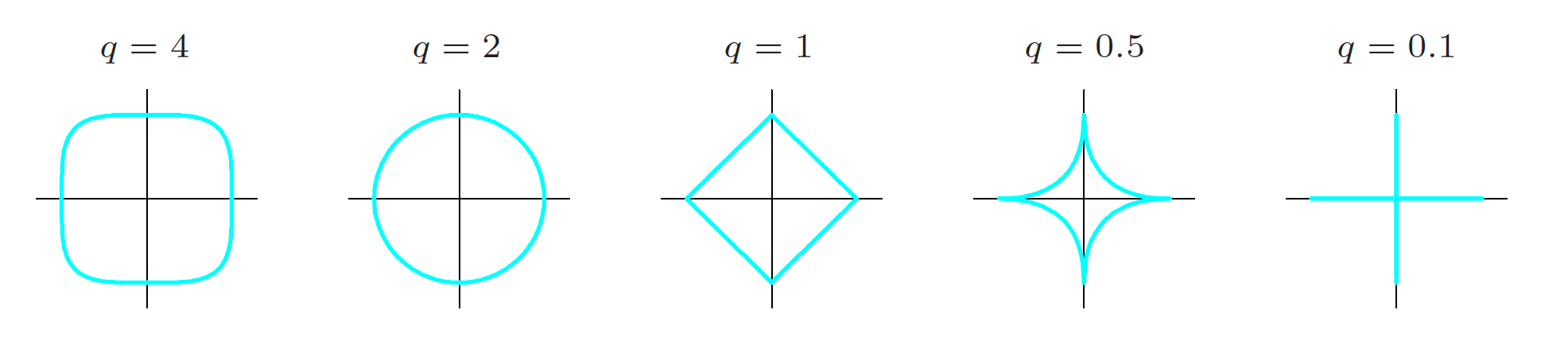
The figure shows contours, or curves of equal value, satisfying $|\beta_1|^q + |\beta_2|^q = 1$.
-
As $q$ tends toward zero, the penalty behaves more like $|\beta_1|^0 + |\beta_2|^0$.
-
For $q \geq 1$, the corresponding regions are convex sets.
-
For $q > 1$, the boundaries intersect the axes smoothly.
Regularization
The following optimization problem is referred to as $\ell_q$ regularized regression for $q \geq 0$:
\begin{align*} \underset{\beta}{\arg\min}\;\; \sum_{i=1}^n\left(y_i - \left(\beta_0 + \sum_{j=1}^p \beta_j x_{ij}\right)\right)^2 + \lambda \sum_{j=1}^p |\beta_j|^q \end{align*}Importantly, for $q \geq 1$, the objective function is convex in $\beta$.
Regularization
-
Implication: it can be solved efficiently to optimality.
-
Rather than resorting to heuristics for best-subset selection, this changes the form of the complexity penalty in a computationally tractable way.
-
As before, we do not penalize the intercept, since it simply finds the right vertical level for the line of best fit.
Most common in practice are $\ell_1$ and $\ell_2$ regularized regression, better known as LASSO and ridge regression.