STATS 413: Lecture 22
-
Criterion-based methods
-
Sample-splitting
Criterion-Based Methods
Alternative approaches to model selection imagine optimizing an objective function which encourages model fit while penalizing model complexity.
We know that if we consider
\begin{align*} \underset{\text{all models}}{\arg\min}\;\; \sum_{i=1}^n(y_i-\hat{y}_i)^2, \end{align*}we'll return the ordinary least squares regression using all $p$ predictors.
Criterion-Based Methods
Consider instead
\begin{align*} \underset{\text{all models}}{\arg\min}\;\; Criterion, \end{align*}We instead minimize a criterion that:
-
Is decreasing as quality of the fit to the observed data increases.
-
Is increasing in the complexity of the model ($m$, the number of included predictors).
Comparing the Criteria
Here are our four suggested criteria to minimize:
-
Based on Adjusted $R^2$: $SSE(\mathcal{M}_m)/(n-m-1)$
-
Mallows' $C_p$: $SSE(\mathcal{M}_m)/\hat{\sigma}^2_\varepsilon(\mathcal{M}_p) + 2(m+1)-n$
-
AIC: $n\log_e\{SSE(\mathcal{M}_m)/n\} + 2m$
-
BIC: $n\log_e\{SSE(\mathcal{M}_m)/n\} + \log_e(n)m$
Comparing the Criteria
For a fixed model size $m$, all of these criteria would agree on the same "best model":
-
Model of size $m$ that yields the smallest $SSE$.
Difference: the nature of the penalty for complexity, namely the penalty on $m$.
Best Subset Selection with Complexity Penalization
For a chosen criterion, if we could evaluate all possible models:
-
For a given model size $m$, evaluate all $\binom{p}{m}$ models of size $m$ and find the set of $m$ predictors yielding the best value for the criterion. Call it $Criterion^*_m$.
-
All four criteria we've introduced would agree upon the best model of size $m$.
-
-
Across values for $m$, find the minimal value for $Criterion^*_m$.
-
This is where the differences between criteria would show up. Different penalizations on $m$ yield different models.
-
This general idea is called Best Subset Selection. Why can't we always implement it?
Extended Diabetes Data
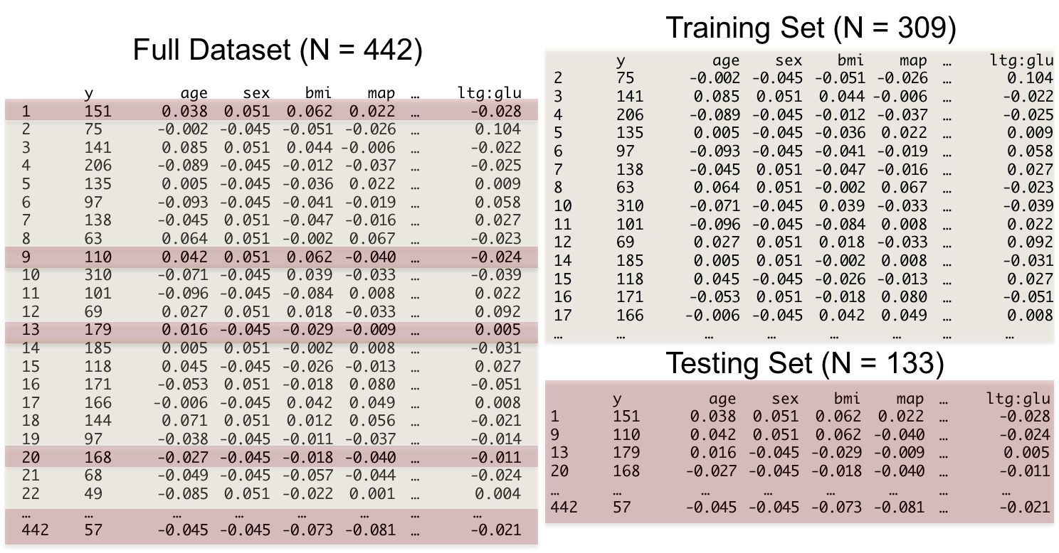
We have data on diabetes disease progression for $n=442$ individuals, along with $p=10$ predictor variables. Suppose we consider using polynomial regression to accommodate potential nonlinearities with respect to our predictor variables.
-
Consider a second degree polynomial: linear, square, and interaction terms.
-
10 baseline variables (Age, Sex, BMI...)
-
45 "interaction" variables such as BMI x Age, etc.
Extended Diabetes Data
-
9 squared variables (we don't include the square of sex; what's the square of a binary?)
-
All covariates are then $z$-scored, so each column has mean zero and standard deviation one.
-
We have $p=10+45+9 = 64$ covariates.
How many possible models are there?
Computation Time For Extended Diabetes Data

Heuristics for Best Subsets
As you can see, explicitly solving the best subset selection problem becomes computationally challenging for $p$ moderate or large.
-
Many real-world data sets have $p >> 64$.
Suggests finding greedy heuristics for the above schema, obviously suboptimal but hopefully computationally tractable.
-
What algorithms might allow us to approximate best subset selection while being usable in practice?
Iterative Model Building
An instinct may be to employ an iterative model building schema to explore the set of all possible models, just like we did with the hypothesis test based approaches.
Common in practice, known as stepwise regression.
Iterative Model Building
Three contenders:
-
Forward Selection: start with a small model with $m=0$ predictors, sequentially grow the model by adding covariates using a pre-specified criterion.
-
Backwards Elimination: start with all covariates, $m=p$, and then sequentially remove covariates using a pre-specified criterion.
-
Hybrid Elimination: a mix of the two, which can be helpful under multicollinearity.
Forward Selection
Let $\mathcal{M}^*_0$ be the initial model with no covariates, so it only includes the intercept. For $m=1,\dots,p$:
-
For each of the variables not included in $\mathcal{M}^*_{m-1}$, consider a new model of size $m$ which adds that particular variable to $\mathcal{M}^*_{m-1}$.
-
Among these candidate new models, let $\mathcal{M}^*_{m}$ be the model with $m$ predictors resulting in the best value for the complexity-adjusted criterion.
-
Calculate the complexity-adjusted criterion for $\mathcal{M}^*_{m-1}$ and $\mathcal{M}^*_{m}$.
-
If the criterion improved, store $\mathcal{M}^*_{m}$ as the new model and continue with the algorithm by considering adding another variable.
-
Otherwise, stop. Return the model $\mathcal{M}^*_{m-1}$.
Backwards Elimination
Let $\mathcal{M}^*_p$ be the initial model with all $p$ covariates included. For $m=p-1,\dots,0$:
-
For each of the variables included in $\mathcal{M}^*_{m+1}$, consider a new model of size $m$ which removes that variable from $\mathcal{M}^*_{m+1}$ while keeping all other variables in $\mathcal{M}^*_{m+1}$.
-
Among these candidate new models, let $\mathcal{M}^*_m$ be the model that minimized the criterion of interest.
-
Calculate the complexity-adjusted criterion for $\mathcal{M}^*_{m+1}$ and $\mathcal{M}^*_m$. If the criterion improved, store $\mathcal{M}^*_m$ as the new model and continue with the algorithm by considering deleting another variable.
-
Otherwise, stop. Return the model $\mathcal{M}^*_{m+1}$.
Hybrid Elimination
Hybrid elimination combines backwards and forwards steps. At each step:
-
Consider all possible models attained by adding a predictor to the existing model.
-
Consider all possible models attained by removing a given predictor from the existing model.
-
Make whatever change results in the smallest value for the complexity-adjusted criterion.
A Reminder: What's the Point?
The point of our enterprise has been to account for the bias-variance tradeoff when deciding how complex to make our model.
-
Issue: sometimes increased complexity can lead to our prediction error increasing when trying to use our data set to make predictions for new observations.
-
Solution so far: incorporate complexity penalties when comparing models of different size.
-
A sensible, and theoretically motivated, attempt to protect against the dangers of overfitting.
A Reminder: What's the Point?
Towards a New Assessment
Might there be a better way to estimate how well a given model would do when faced with new data?
Training and Test Sets
How might we use our given data set to mimic predictive performance on new data?
-
Answer: sample splitting.
Imagine taking our data set with $n$ observations, and randomly splitting it into two mutually exclusive/disjoint and exhaustive sets:
-
A training set of size $n_{train}$.
-
A test set of size $n_{test}$.
-
We typically choose $n_{train} > n_{test}$.
-
For a prediction task, a 70-30 split might be reasonable.
Training and Test Sets
After creating this partition:
-
Build a predictive model using only the training set.
-
Evaluate its performance by how well it can predict the observations in the test set.
Training and Test Set (Random Split)
-
We refer to performance metrics defined using the training set as in-sample.
-
Metrics based on the test set are out-of-sample.
Out-of-Sample $R^2$
We can define a better $R^2$ by using our training data to predict our test data. Recall that we motivated $R^2$ as a metric for improvement relative to a baseline model that only predicted the mean for all individuals.
-
Based on our training set, our best guess for the population mean is $\bar{y}_{train}$, which is what we'd predict for everyone in the test set under this simple model.
-
Based on our training set, we predict $\hat{y}_i = \hat{f}(x_i)$ for individual $i$ in the test set.
Out-of-Sample $R^2$
Out-of-Sample $R^2$
\begin{align*} OSR^2 &= 1-\frac{\sum_{i=1}^{n_{test}}(y_i - \hat{y}_i)^2}{\sum_{i=1}^{n_{test}}(y_i - \bar{y}_{train})^2} \end{align*}Extended Diabetes Regression Model
| Algorithm | Model Size ($m$) | $R^2$ | $OSR^2$ |
|---|---|---|---|
| Full Model | 64 | 0.631 | 0.340 |
| AIC, backward | 23 | 0.611 | 0.335 |
| BIC, backward | 14 | 0.585 | 0.358 |
| AIC, forward | 14 | 0.587 | 0.370 |
| BIC, forward | 5 | 0.537 | 0.416 |
Extended Diabetes Regression Model
-
Should be no surprise that the full model did best in-sample.
-
BIC, forward gave the best $OSR^2$.
-
Also provided the most parsimonious, simple model.
-
A 5 variable model that does better out of sample than a 64 variable model.
-
Could models with better $OSR^2$ exist?
Information Criterion
Our Information Theory criteria were:
-
Akaike Information Criterion: $AIC(\mathcal{M}_m) = n\log_e(SSE(\mathcal{M}_n)/n) + 2m$
-
Bayesian Information Criterion: $BIC(\mathcal{M}_m) = n\log_e(SSE(\mathcal{M}_n)/n) + \log_e(n)m$
Information Criterion
So they are generally of the form
\begin{align*} Crit_\lambda(\mathcal{M}_n) &= n\log_e(SSE(\mathcal{M}_n)/n) + \lambda m, \end{align*}for different choices of $\lambda$.
-
Could we have uncovered a model with better $OSR^2$ with a different choice of $\lambda$? Absolutely.
-
Can we consider choosing $\lambda$ intelligently? Yes.
Intuition for Optimizing Over $\lambda$
Targeting the following optimization problem to choose our model:
\begin{align*} \underset{\text{all models}}{\arg \min} Crit_\lambda(\mathcal{M}_n) &= n\log_e(SSE(\mathcal{M}_n)/n) + \lambda m, \end{align*}for different choices of $\lambda$.
-
Set $\lambda = 0$ with no penalty, and this returns the full model including all variables.
-
Low bias, high variance: overly complex and includes irrelevant predictors.
-
-
Send $\lambda \rightarrow \infty$, and this returns a model that only includes an intercept.
-
Low variance, high bias.
-
Intuition for Optimizing Over $\lambda$
Different choices of $\lambda$ result in different trade-offs between bias and variance.
-
Optimizing $\lambda$ means finding the right trade-off between bias and variance for a given problem.
A Fundamental Picture
-
In general, as the model complexity increases, errors in forming predictions for the observed data will decrease, which is the same as maximizing in-sample $R^2$.
-
However, errors for future observations can increase with too much complexity because of fitting to noise.
-
Different choices of $\lambda$ help us navigate the bias-variance tradeoff, ideally finding the optimal point on the out-of-sample curve.
A Fundamental Picture

A Seemingly Sensible Approach
Here's a seemingly innocuous approach, catered to forward stepwise. For a grid of values of $\lambda$:
-
Run forward stepwise on the training set, and use $Crit_\lambda$ as our complexity penalized metric.
-
Evaluate the performance for each $\lambda$ on the test set.
-
Choose the $\lambda$ that maximizes performance on the test set.
What's Wrong?
The issue with the previous approach is that it corrupts the nice properties of our out-of-sample $R^2$.
-
When we didn't optimize over $\lambda$ and instead fixed it beforehand, the $OSR^2$ truly did reflect a measure of performance on future observations, and we could compare values of $OSR^2$ in choosing a model.
Optimizing over $\lambda$ as we've done it forms a link between the training sets and test sets.
What's Wrong?
-
The test set is meant for validation, but now it's being used to inform the prediction strategy.
-
Properties of the test set have bled into the choice of prediction function $\hat{f}$, such that the two sets of observations are related.
-
It would be unfair to compare forward stepwise with $\lambda$ optimized in this way to, say, backwards elimination based upon Adjusted $R^2$. One had access to the test set, the other did not.
Choosing Tuning Parameters
Leads to what is known as an optimism bias.
-
The $OSR^2$ at the value of $\lambda$ that maximizes test set $OSR^2$ will be larger, on average, than what the $OSR^2$ would be when faced with future data.
-
The optimal $\lambda$ was chosen to do best on the test set. In a sense, it might overfit to the test set.
-
Gives an unfair advantage in certain model comparisons.
Choosing Tuning Parameters
For instance, imagine comparing the performance at the best $\lambda$, chosen by looking at the test set, to the performance of a model chosen by consulting outside experts before looking at the data.
-
If we choose the covariates in the model before looking at the data, we do this in a way that is truly blind to the test set.
-
The optimal $\lambda$ would instead look at the test set to inform the chosen value of $\lambda$.
Choosing Tuning Parameters
Many statistical methods have tuning parameters, or hyperparameters, associated with them.
Issue: we cannot simultaneously:
-
Use the test set to choose the best value for them.
-
Use the test set to estimate out of sample performance of an algorithm given the optimized tuning parameters.
Particularly important to choose tuning parameters in a better way if we are:
-
Comparing algorithms with different tuning parameters.
-
Comparing an algorithm with a tuning parameter to one without.
A First Solution: Include a Validation Set
A simple solution to the above would be to include a third split: a validation set.
-
Partition the data set three ways: training, validation, test.
-
60-20-20 might be reasonable.
Consider, for a given algorithm:
-
Use the training set to come up with a model, while optimizing tuning parameters based on predictive performance on the validation set.
-
Once the optimal tuning parameters have been chosen, evaluate out-of-sample predictive performance on the test set.
A First Solution: Include a Validation Set
Since the test set has been kept out of the selection process, this scheme does give trustworthy out-of-sample performance estimates and removes optimism bias.
Downsides of a Validation Set
While this would work, it may seem like we're sacrificing a lot of data just for the sake of estimating a tuning parameter.
-
We're losing data for coming up with our predictive model, and we're also losing data for evaluating predictive performance.
Might there be a more data-conscious way of proceeding that adheres to the spirit of a validation set? Stay tuned...