STATS 413: Lecture 20
-
Regression splines
-
Natural splines
-
Generalized additive models
Deficiencies in Polynomials
As a means of capturing nonlinear trends, polynomials suffer from a few important deficiencies:
-
The only way to fit increasingly complex functions is to increase the polynomial degree.
-
Individual observations affect the prediction function globally. Changes in the response in one region of the domain of $x$ can substantially impact the polynomial's behavior in other regions.
Deficiencies in Polynomials
-
Polynomials are particularly prone to being influenced by outliers.
-
Adapting to varying trends in varying regions of $x$ can require high-degree polynomials, which introduce instability through high variance.
-
Behavior at the boundary can be highly unstable, often with oscillation and perfect interpolation.
A Challenging Example for Polynomial Regression
A Challenging Example for Polynomial Regression
Each data point affects the fit globally. The polynomial must trade off performance in the center and at the extremes, even with a large degree.
Piecewise Polynomials
Sometimes the nonlinear pattern can change substantially across different regions of $x$.
-
Example: modeling demand for Uber as a function of hour of day, and comparing the late morning to the evening commute.
Should this occur, a single polynomial fit would likely be inadequate.
-
Low polynomial degree: bias may remain.
-
High polynomial degree: too much variance.
Piecewise Polynomials
Rather than fitting one polynomial over all values of $x$, we might fit different low-degree polynomials over different ranges of $x$.
\begin{align*} y_i &= \begin{cases} \beta_{01} + \beta_{11}x + \beta_{12}x^2 + \beta_{13}x^3 + \varepsilon_i & x \leq \xi_1\\ \beta_{02} + \beta_{12}x + \beta_{22}x^2+\beta_{23}x^3 + \varepsilon_i & \xi_1 < x \leq \xi_2\\ \beta_{03} + \beta_{13}x + \beta_{23}x^2 + \beta_{33}x^3 + \varepsilon_i & \xi_2 < x \leq \xi_3\\ \beta_{04} + \beta_{14}x + \beta_{24}x^2 + \beta_{34}x^3 + \varepsilon_i & x > \xi_3 \end{cases} \end{align*}Drawbacks of Piecewise Polynomials
The drawbacks of piecewise polynomials are readily apparent once we look at the prediction equation.
-
The fit is discontinuous at the boundaries $\{\xi_k\}$.
-
We generally imagine the function we are estimating is continuous over the domain of $x$.
While piecewise polynomials are rarely deployed in practice, they motivate a family of commonly used methods known as splines.
-
Splines are based on piecewise polynomials while imposing constraints to ensure continuity and smoothness.
Regression Splines
Instead of fitting a high-dimensional polynomial over the entire range of $x$, a regression spline fits different low-dimensional polynomials over different regions of $x$.
-
For example, a cubic spline fits $f(x)=ax^3+bx^2+cx+d$, but the coefficients may differ depending on the value of $x$.
The $K$ points where the coefficients change, $\xi_1,\dots,\xi_K$, are called the knots, or breakpoints, of the spline.
-
More knots means more flexibility.
-
Higher polynomial degree in each region also means more flexibility.
-
More flexible is not always better; it can lead to overfitting.
Regression Splines
Unlike piecewise polynomials, splines are constructed using piecewise polynomials of degree $d$ such that the resulting fit is smooth at the knots $\xi_1,\dots,\xi_K$.
-
Suppose I fit a regression spline using a degree $d$ polynomial.
-
Then, at each knot $\xi_k$, the function will be continuous at $x = \xi_k$.
-
In addition, all derivatives $f^{(1)},\dots,f^{(d-1)}$ will also be continuous at $x=\xi_k$ for $k=1,\dots,K$.
-
Continuity of derivatives provides additional smoothness.
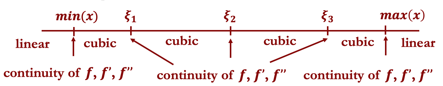
Cubic Spline
Example: an estimated cubic spline will be continuous at all $K$ knots. In addition, the first and second derivatives will also be continuous at $x = \xi_k$, $k=1,\dots,K$.

Ensuring Smoothness in the Spline Fit
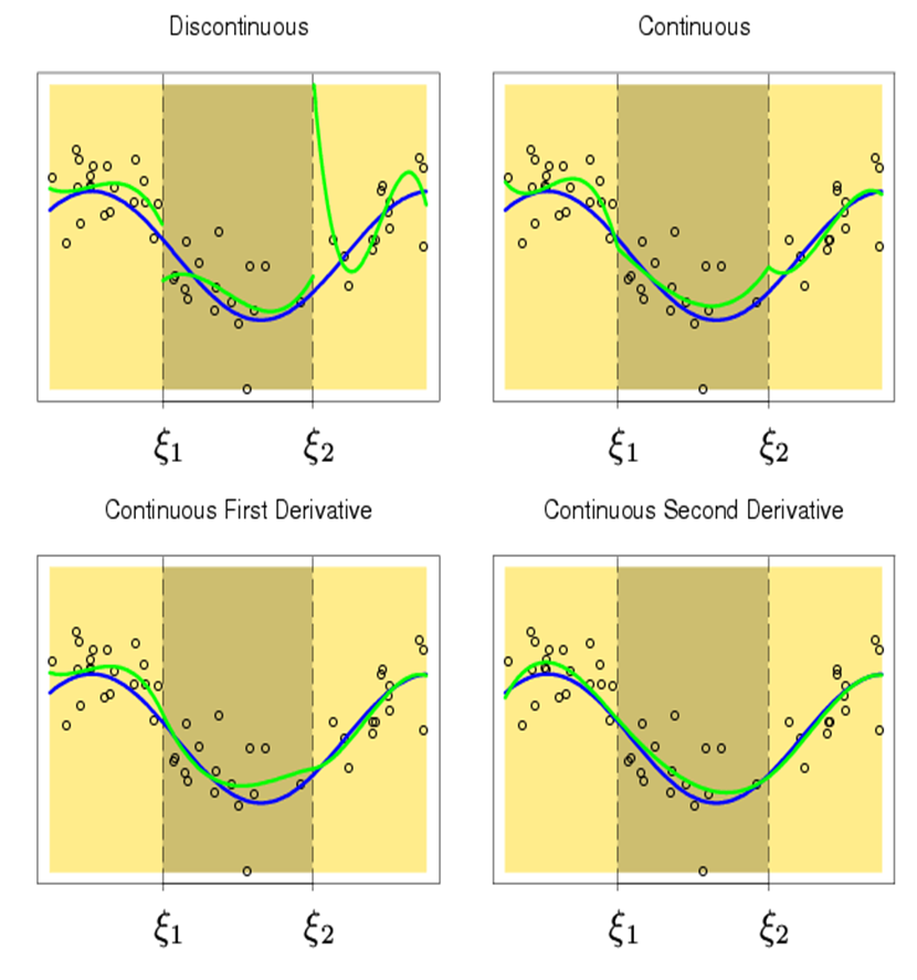
The Number of Free Parameters
In the figure above, it may appear as though there are $4 \times 4$ free parameters to choose.
-
There are $K=3$ knots, resulting in $K+1=4$ regions.
-
Each region gets its own polynomial. For a cubic, $d=3$, this involves an intercept plus coefficients on the linear, squared, and cubed terms. That gives $d+1=4$ parameters per region.
The Number of Free Parameters
However, our continuity and smoothness requirements impose constraints.
-
For each knot, there are $d$ constraints: one for continuity and $d-1$ for smoothness. In this example, $d=3$ gives three constraints per knot.
-
Total constraints across knots: $K \times d$, or $3 \times 3$ in this example.
Free Parameters for Regression Splines
For a degree $d$ spline with $K$ knots, the number of parameters we get to choose is
\begin{align*} df &= (K+1)(d+1) - Kd\\ &= Kd + K + d + 1 - Kd\\ &= K + d + 1 \end{align*}Think of $K+d$ as the analogue of $p$ in the usual regression setting, with an additional intercept term.
-
Cubic spline: $K+d+1=K+4$ parameters. One for the intercept, and $K+3$ more for the rest of the cubic spline.
Location of Knots
The knot locations $\xi_1,\dots,\xi_K$ can be pre-specified by the user if there are known areas in the domain of $x$ that represent different regimes in the problem.
If we do not have that knowledge and simply want to fit a spline with $K$ knots, two natural defaults arise in practice.
-
Equi-spaced knot points, so the knots are the same distance apart.
-
Knots based on quantiles of $x$, so each of the $K+1$ regions contains the same fraction of observations. This is the most common choice and is built into
R.-
If $K=3$, put knots at the 25th, 50th, and 75th percentiles of $x$.
-
Regression Splines in Challenging Example
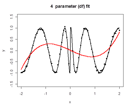
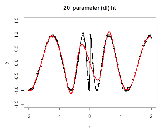
Regression Splines in Challenging Example
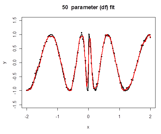
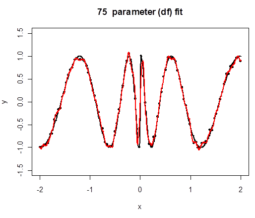
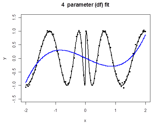
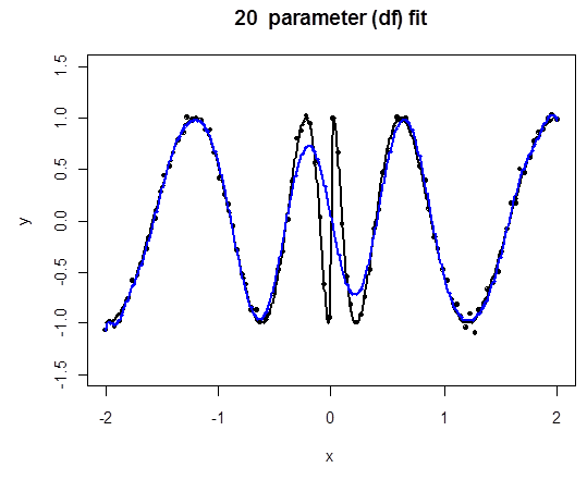
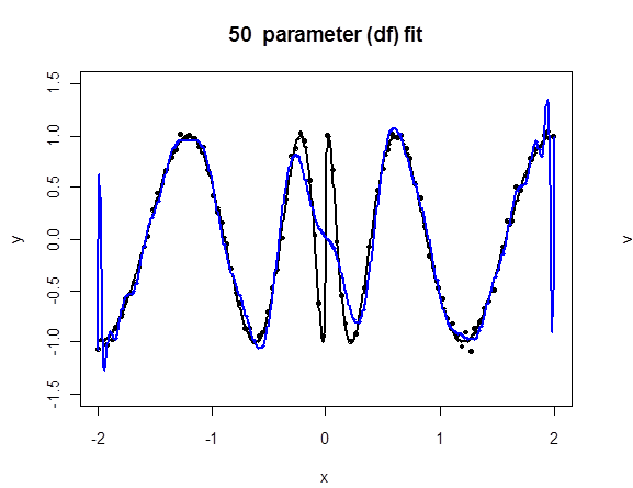
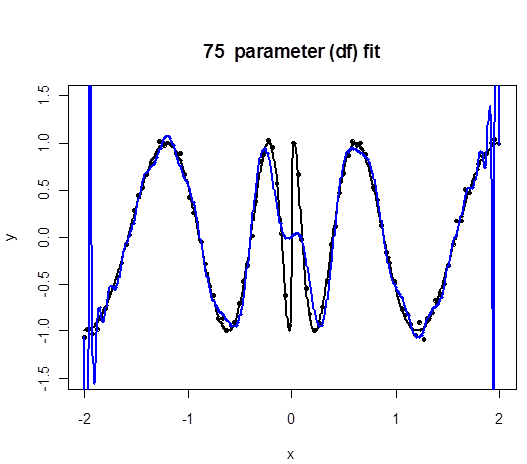
Here we fit cubic splines to the original problematic example and increase the number of knots $K$. Twenty parameters means sixteen knots.
Spline vs Polynomial Comparison
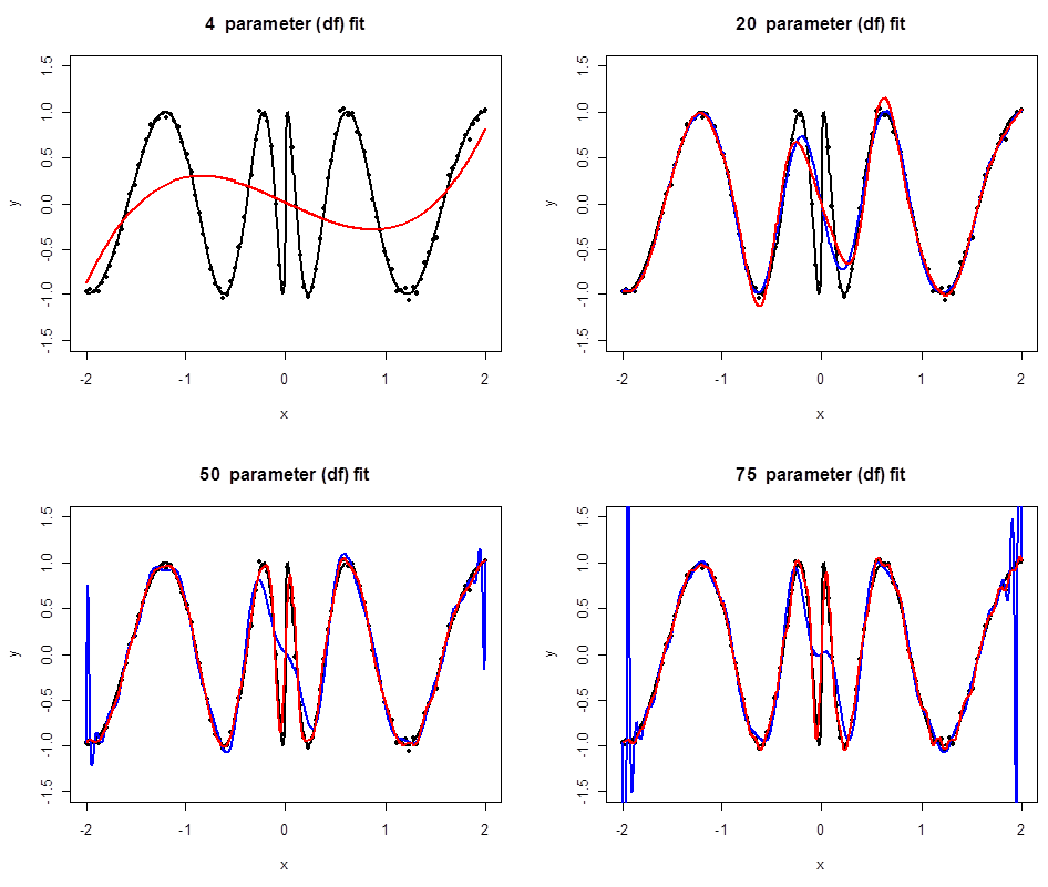
Spline vs Polynomial Comparison
Polynomial regression, in blue, increases degrees of freedom by increasing polynomial degree.
Regression splines, in red, keep cubic pieces but increase the number of knots, which lets the spline adapt more effectively to curvature.
Regression Splines in Practice
By far, the most common type of regression spline is a cubic spline.
-
Higher degrees can produce smoothness that is hard to discern by eye, while also creating instability and wobbly functions.
-
Knot points $K$ are the primary way complexity is controlled.
-
Knot locations should be chosen with out-of-sample performance in mind.
-
Typically, though not always, cubic regression splines outperform polynomial regression.
-
Increasing complexity by adding knots tends to be more stable than increasing polynomial degree.
Basis Functions
Both polynomial regression and regression splines are members of a broad class of regression methods that use basis functions.
-
Idea: have a pre-specified family of functions or transformations that can be applied to a predictor $x$, namely $\{b_1(x),\dots,b_r(x)\}$.
-
Then fit a model of the form
Basis Functions
Ex: instead of writing a polynomial regression of degree $r$ as
\[ y_i = \beta_0 + \beta_1 x_i + \beta_2 x_i^2 + \cdots + \beta_r x_i^r + \varepsilon_i \]we can write it as
\[ y_i = \beta_0 + \beta_1 b_1(x_i) + \beta_2 b_2(x_i) + \cdots + \beta_r b_r(x_i) + \varepsilon_i, \]where $b_j(x_i) = x_i^j$.
Other Basis Functions
-
Once you write the model this way, you can imagine many other options for the basis functions $b_j(x_i)$.
-
Notice that once you choose the basis functions, you can just use ordinary least squares to estimate the $\beta$'s, so this approach is very easy to implement.
-
There are in fact many different bases used in practice, such as wavelets and Fourier series.
Regression Splines Represented Using Basis Functions
We can also represent a cubic spline with $K$ knots using the basis-function representation
\[ y_i = \beta_0 + \beta_1 b_1(x_i) + \beta_2 b_2(x_i) + \cdots + \beta_{K+3} b_{K+3}(x_i) + \varepsilon_i, \]where $b_0(x)=1$, $b_1(x)=x$, $b_2(x)=x^2$, $b_3(x)=x^3$, and
\begin{align*} & b_{j+3}(x)=(x-\xi_j)_+^3 = \begin{cases} 0 & x \leq \xi_j\\ (x-\xi_j)^3 & x > \xi_j \end{cases}\quad j=1,\ldots,K \end{align*}-
Once we have $b_j(x_i)$ for each $x$, we can use ordinary least squares to estimate the $\beta$'s and hence fit the spline.
Deficiencies in Regression Splines
Regression splines overcome one of the main limitations of polynomial regression.
-
They fit local piecewise polynomials of small degree, rather than a single polynomial providing a global fit.
That said, regression splines can still exhibit instability at the extremes of the distribution of $x$.
-
The prediction equation can have large variance when $x$ is near the minimum or maximum value of the variable.
-
This occurrence is called a boundary effect, and it is common with many nonlinear methods.
Can we mitigate this issue?
Natural Splines
Natural splines are a slight modification of cubic regression splines that improve stability at the boundary. If we have $K$ knots:
-
The fit is still piecewise cubic in all $K-1$ interior regions between knot points.
-
It is also piecewise cubic between $\min(x)$ and the smallest knot point, and between the largest knot point and $\max(x)$.
Natural Splines
-
We further enforce that the prediction function becomes linear once it goes outside the range $[\min(x), \max(x)]$.
-
Forcing the function to be linear while extrapolating is where natural splines differ from cubic regression splines.
Natural Splines
-
At the boundary points $\min(x)$ and $\max(x)$, we enforce continuity of the piecewise functions and also continuity of the first and second derivatives.
-
The prediction function must therefore have second derivative equal to zero at the boundary, since a line has zero second derivative.
-
This results in a total of $K+2$ parameters to choose.
Natural Splines and Boundary Effects
Why can natural splines improve stability at the boundary?
-
A cubic function is more complex than a line.
-
As we've learned, more complexity in an estimated function results in additional variability across data sets.
-
Enforcing linear behavior at the boundary introduces more stability, since a line is less complex than a cubic.
-
It can also introduce more bias for the same reason, but the hope is that we trade bias for variance effectively.
Dealing with Multiple Predictors
Our discussion so far has focused on a single predictor variable.
-
What if we have $p>1$ predictors?
In general, we'd be interested in fitting functions of the form
\[ y_i = f(x_{i1},\dots,x_{ip}) + \varepsilon_i, \]where $f$ is unknown.
We discussed polynomial regression with $p>1$ at the end of the last lecture as one way to approximate this.
-
That becomes difficult in general without making further assumptions about the functional form of $f(\cdot)$.
Generalized Additive Models
When we have several predictors and want a nonlinear fit by extending univariate methods, a natural extension of multiple linear regression
\[ y_i = \beta_0 + \beta_1 x_{i1} + \beta_2 x_{i2} + \cdots + \beta_p x_{ip} + \varepsilon_i \]is to replace each linear part, $\beta_j x_{ij}$, with $g_j(x_{ij})$ where $g_j$ is a smooth nonlinear function.
We would then write the model as
\[ y_i = \beta_0 + g_1(x_{i1}) + g_2(x_{i2}) + \cdots + g_p(x_{ip}) + \varepsilon_i \]Assumption: there are no interaction terms of the form $h_1(x_{i1},x_{i2})$ or $h_2(x_{i1},x_{i2},x_{i3})$ unless we add them explicitly.
GAMs
This model is an example of a Generalized Additive Model.
-
It is called additive because we calculate a separate $g_j$ for each $x_j$ and then add them all together.
In general, we represent each $g_j(x_j)$ through a flexible basis expansion.
-
One could let $g_j(\cdot)$ be a polynomial of a specific degree in $x_j$.
-
Perhaps the most common approach is to let $g_j(\cdot)$ be a spline in $x_j$ for each $j=1,\dots,p$.
The Boston Housing Data
The Boston Housing data set contains information collected by the U.S. Census Bureau concerning housing around Boston in the 1970s.
-
Response: median housing price in a given census tract.
-
Covariates: 13 variables including per-capita crime, pupil-teacher ratio, proximity to highways, and more.
The data were originally collected to assess the impact of air quality on housing prices.
-
It has since become a benchmark data set for machine-learning algorithms.
Comparing Two Approaches
To illustrate the potential benefit of GAMs for out-of-sample prediction, split the data into training and test sets. In the training set, fit:
- Linear regression using all 13 covariates.
- A GAM using natural splines with 5 knots each.
The GAM is based on only four of the 13 variables:
- Crime rate.
- Industrial proportion.
- Median number of rooms per dwelling.
- Proportion of individuals in lower socioeconomic strata.
Ex: Impact of Lower Socioeconomic Strata
Holding the other variables at their mean values, this plot shows the predicted median values for homes as we vary the proportion of lower-status individuals.

A Comparison
Here is the out-of-sample $R^2$ for the two models.
| Method | $R^2$ on the test set |
|---|---|
| Linear regression with 13 covariates | 0.645 |
| GAM with 4 covariates | 0.719 |
By allowing for nonlinearities through a GAM, we were able to improve out-of-sample performance.
Pros of GAMs
-
By allowing a nonlinear $g_j$ for each $x_j$, we can automatically model nonlinear relationships that standard linear regression will miss.
-
As the housing example shows, this can potentially yield more accurate predictions.
-
Because we are fitting an additive model, we can still examine the effect of each $x_j$ on $y$ while holding the other predictors fixed.
-
Hence, if we care about interpretation of particular covariates, GAMs can be appealing.
Cons of GAMs
-
The model is restricted to be additive in the terms $g_j(x_j)$.
-
Thus the fit is not completely nonlinear.
-
A simple interaction of the form $y = x_1x_2 + \varepsilon$ cannot be captured automatically by a GAM.
-
We can still manually add interaction terms, but that requires an active modeling choice.
-
More complicated methods can learn nonlinearities and interactions automatically, but they are not really linear models.