STATS 413: Lecture 19
-
Bias-variance tradeoff
-
Training and test evaluations
Recap: An Exercise in One Dimension
Suppose we are presented with the following data set, and are asked to come up with a predictive model for $y$ as a function of $x$.

Recap: An Exercise in One Dimension
It's clearly not linear. Instead, it seems that $y_i = f(x_i) + \varepsilon_i$ for some nonlinear function $f(\cdot)$.
-
What was polynomial regression? How do we implement it?
Approximations of Increasing Polynomial Degree

Performance Assessment
-
If I fit polynomials of degrees $1,2,\dots,15$, which prediction equation will provide the smallest $SSE$ or, equivalently, the largest $R^2$ for our observed data set?
-
Should we always use the prediction method that yields the largest $R^2$?
-
What was prediction error? Did it refer to accuracy for our observed data, or for future observations?
An Illustration of Prediction Error: Fitting a Line When Truth is Quadratic
Suppose we fit a line, $\widehat{f}(x) = \widehat{\beta}_0 + \widehat{\beta}_1x$ when, in reality, $f(x) = \gamma_0 + \gamma_1 x + \gamma_2 x^2$.

See the R script from last lecture for the corresponding simulation.
On Reducing Reducible Error
Prediction error can be decomposed into three terms:
On Reducing Reducible Error
The last two terms are the ones we can hope to control based on how we estimate $\widehat{f}(\tilde{x})$.
-
Ideally, we'd like to minimize both terms.
-
Unfortunately, strategies that minimize one term need not minimize the other.
Targeting One, Not the Other
Stupid Example 1: Suppose I decide, "My favorite number is 5, so I'm going to predict $\widehat{f}(x) = 5$ regardless of $x$ and no matter how the data looks."
-
What would the estimator variance be?
-
What about estimator bias?
Targeting One, Not the Other
Stupid Example 2: Suppose my data $y_1,\dots,y_n$ are iid with common mean $\mu$ and variance $\sigma^2 = 1$, so there are no covariates. As an estimator for a future observation $y_i^*$, I consider choosing $\widehat{f} = y_1$.
-
What would the estimator's bias be?
-
What about the estimator's variance?
-
Compare the reducible error of this estimator to that of $\widehat{f} = \bar{y} + 1/\sqrt{n}$ for $n \geq 2$.
The Bias-Variance Tradeoff
Here's what we saw last class with $RMSE$ for future observations in our polynomial simulation.

The Bias-Variance Tradeoff
What's going on?
-
Increasing the polynomial degree decreases bias because we are getting better approximations of the true function.
-
Increasing the polynomial degree increases variance, as we begin to fit too much to noise and overfit.
This is a general phenomenon known as the bias-variance tradeoff.
The Bias-Variance Tradeoff
The Bias-Variance Tradeoff
As a general rule, as we increase model complexity, estimator bias decreases while estimator variance increases.
The takeaway: we need to think of ways to find an optimal tradeoff between the two.
A Fundamental Picture
-
In general, as model complexity increases, errors in forming predictions for the observed data decrease.
-
Errors for future observations will decline at first, as reductions in bias dominate, but then start to increase again, as increases in variance dominate.
A Fundamental Picture
-
We must always keep this picture in mind when choosing a model. More flexible or complicated is not always better.

The Tradeoff with $n$ Large
As the sample size increases, the bias and variance of an estimator behave differently. For a fixed degree of complexity:
Bias doesn't change much as $n$ increases.
-
Bias has to do with misspecification of the true function.
-
Even with $n = 10^{10}$, I'm still in trouble if I try to fit a line to a relationship that is quadratic.
The Tradeoff with $n$ Large
Variance of an estimator does decrease as $n$ increases.
-
Think of this in analogy to $\text{Var}(\bar{y}) = \sigma^2/n$.
-
The rate at which an algorithm's variance decreases can vary, but typically any reasonable prediction function's variance will tend to zero.
Bias Dominates with $n$ Large
Again, here's our decomposition:
\[ \text{Prediction Error} = \text{Irreducible Error} + \text{Squared Bias} + \text{Variance} \]-
Irreducible error doesn't change as $n$ increases.
-
For a fixed degree of complexity, squared bias doesn't predictably decrease or increase.
-
For a fixed degree of complexity, variance decreases.
So for sufficiently large sample sizes, the reducible error is dominated by the bias.
On Accounting for the Tradeoff
The tradeoff shows us that we must avoid overfitting to data.
-
We cannot naively find the best fitting function to the data set at hand, because we might be fitting to apparent "patterns" that are due to random chance alone.
On Accounting for the Tradeoff
This highlights the deficiencies in $R^2$ as a metric for model performance.
-
It does not account for model complexity at all, and becomes larger and larger with more complex models.
-
It only compares reduction in error within our particular sample.
-
As we compare models of different sizes and complexities, we need to consider performance on future data, rather than on the observed data.
Accounting for Complexity when Choosing a Model
The big issue we're trying to overcome: overfitting.
-
More complex models tend to overfit to noise, especially when the sample size is small, which hurts how well they generalize to new data sets.
-
Comparing models based on $R^2$ doesn't account for this. The more complex model will always win.
Accounting for Complexity when Choosing a Model
Can we develop strategies for choosing between models of different complexity that reflect performance on future observations?
-
We've actually seen one such strategy already under the stronger linear model: partial $\mathcal{F}$-tests. More on this next week.
-
We'll now describe a general strategy for comparing models.
Training and Test Sets
How might we use our given data set to mimic predictive performance on new data?
-
Answer: sample splitting.
Imagine taking our data set with $n$ observations and randomly splitting it into two mutually exclusive and exhaustive sets:
-
A training set of size $n_{train}$.
-
A test set of size $n_{test}$.
-
We typically choose $n_{train} > n_{test}$.
-
For a prediction task, a 70-30 split might be reasonable.
Training and Test Sets
After creating this partition:
-
Build a predictive model using only the training set.
-
Evaluate its performance by how well it can predict the observations in the test set.
Test Set and New Data
Essential: in this setup, the test set cannot play any role in building the prediction algorithms.
-
It needs to truly act as though it was new, as-yet unseen data.
-
Prediction models fit in the training set need to be independent of the observations in the test set.
Imagine locking the test set away in a box, only to be opened when evaluating different prediction equations fit on the training set.
An Important Qualification
In saying that performance on the held-out test set will reflect performance on future observations, we are making an assumption that is often left unsaid.
-
Future observations must be drawn from the same distribution as present observations.
-
In words, the present must be representative of the future.
An Important Qualification
Imagine training a model in 2006 to predict home prices in 2008.
-
No amount of machine learning based on 2006 data could prepare you for 2008.
-
You effectively have zero data on the process in 2008 because it was so different from that in 2006.
This issue is known as generalizability of a model. Can it be used outside of the snapshot in time from which the data arose?
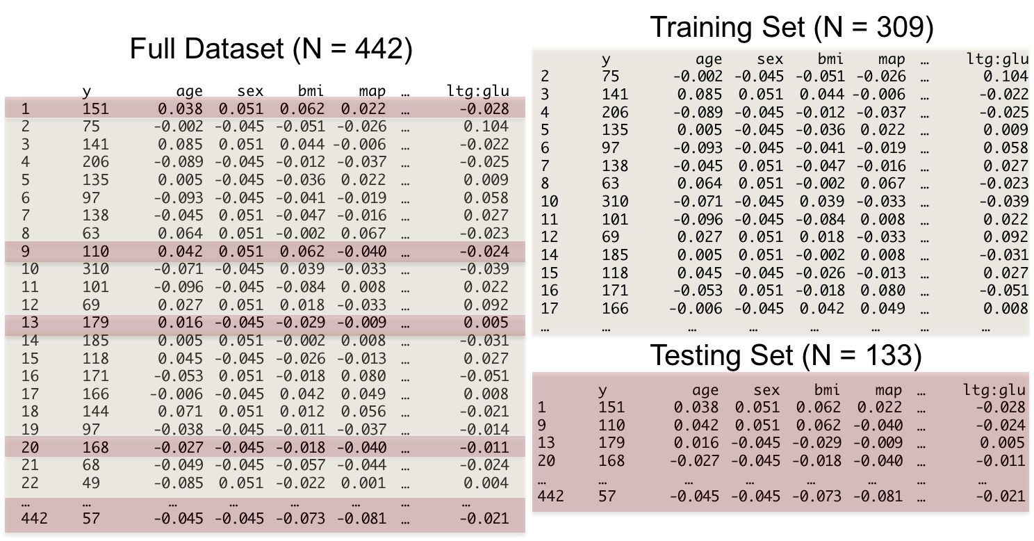
Training and Test Set (Random Split)
-
We refer to performance metrics defined using the training set as in-sample.
-
Metrics based on the test set are out-of-sample.
Example: Out-of-Sample RMSE
Suppose, based only on our training set, we fit a predictive model.
-
$\widehat{f}(\cdot)$ is the resulting prediction equation.
For each of the $n_{test}$ individuals in our test set, we have responses $y_i$ along with their covariates $x_i$.
-
Generate predicted values for the test data based on the model fit to the training set. Call these $\widehat{y}_1,\dots,\widehat{y}_{n_{test}}$.
Example: Out-of-Sample RMSE
Out-of-Sample RMSE
\[ OS\text{-}RMSE = \sqrt{\frac{1}{n_{test}}\sum_{i=1}^{n_{test}}(y_i - \widehat{y}_i)^2} \]This is an estimate of prediction error, since none of the responses in the test set were used to form the predictions $\widehat{y}_i$.
Overfitting
-
Training, or in-sample, $RMSE$ gets very low as complexity increases.
-
Testing, or out-of-sample, $RMSE$ exhibits the bias-variance tradeoff.
Overfitting

Out-of-Sample $R^2$
We could similarly define a better $R^2$ by using our training data to predict our test data.
Recall that we motivated $R^2$ as a metric for improvement relative to a baseline model that only predicted the mean for all individuals.
Out-of-Sample $R^2$
-
Based on our training set, our best guess for the population mean is $\bar{y}_{train}$, which is what we'd predict for everyone in the test set under this simple model.
-
Based on our training set, by exploiting information in $x$ we predict $\widehat{y}_i = \widehat{f}(x_i)$ for individual $i$ in the test set.
Out-of-Sample $R^2$
\[ OSR^2 = 1 - \frac{\sum_{i=1}^{n_{test}}(y_i - \widehat{y}_i)^2}{\sum_{i=1}^{n_{test}}(y_i - \bar{y}_{train})^2} \]An Example: Forced Expiratory Volume Data
We have data on $n=606$ individuals aged 6-17, collected to assess the impact of secondhand smoke from parents on height and lung capacity.
Our variables are:
-
Forced expiratory volume (
FEV), a measure of lung capacity during a forced breath. -
Age.
An Example: Forced Expiratory Volume Data
-
Height.
-
Gender.
-
Whether either parent smokes.
For now we'll just consider the relationship between FEV and age, to see how FEV
develops over time.
Training and Test Set Split
Suppose we randomly split our data set of size $n=606$ roughly 70-30 into a training set and a test set.
-
Explore the data and fit differing-degree polynomials using $n_{train} = 424$ observations.
-
Choose the polynomial degree by evaluating performance on the $n_{test} = 182$ observations in the test set.
Importantly, the test set is not involved in fitting the polynomial regressions.
Visualization on the Training Set

Clear nonlinearity. How many polynomial terms will suffice?
Performance on the Training Set
Here's a graph showing $R^2$ on the training set as a function of polynomial degree.
No surprise: the polynomial with the largest degree has the largest $R^2$ on the training set.

Test Set Evaluation
To account for deficiencies in $R^2$, we should instead evaluate performance on the test set:
-
Fit polynomials of degree $j$ using $y_{train}$ and $x_{train}$. Call the result $\widehat{f}_j(\cdot)$.
-
For each observation $i$ in the test set, calculate $\widehat{y}_i = \widehat{f}_j(x_i)$.
Calculate the out-of-sample $R^2$:
\[ OSR^2(j) = 1 - \frac{\sum_{i=1}^{n_{test}}(y_i - \widehat{f}_j(x_i))^2}{\sum_{i=1}^{n_{test}}(y_i - \bar{y}_{train})^2} \]Out of Sample Performance

Degree 5 polynomial had the best out-of-sample $R^2$.
The Final Model
Once we've chosen the polynomial with the best out-of-sample performance, we:
-
Recombine the training and test sets.
-
Run a polynomial regression on the entire data set using the chosen polynomial degree.
This is especially useful when $n$ is small. For a fixed complexity level, increasing the amount of data results in more stable estimated functions, lowering variance and overall prediction error.
The Result
Here's a scatter plot based on the entire data set, along with the fifth-degree polynomial.

Danger: Extrapolation
While it's always true that we should avoid extrapolation, the issue can be amplified with polynomials.
Here's our fifth-degree polynomial plotted for ages up until 25.

Polynomials in Several Predictors
We can define polynomials with multiple predictor variables.
-
A second-degree polynomial includes linear terms, quadratic terms, and all pairwise interaction terms between variables $x_1,\dots,x_p$.
Example with $p=3$:
\begin{align*} f(x) &= \beta_0 + \beta_1x_1 + \beta_2x_2 + \beta_3x_3 + \beta_4x_1^2 + \beta_5x_2^2 + \beta_6x_3^2 \\ &\quad + \beta_7x_1x_2 + \beta_8x_1x_3 + \beta_9x_2x_3 \end{align*}Polynomials in Several Predictors
-
A third-degree polynomial includes linear, quadratic, cubic, plus interactions of the form $x_1x_2$, $x_1x_2x_3$, and $x_1^2x_2$.
-
A fourth-degree polynomial is, naturally, even messier.
For even moderate $p$, the number of polynomial terms explodes quickly once we move to third degree or higher.
-
In practice, people rarely go beyond a second-degree polynomial with multiple predictors, especially when $p$ is moderately large.