STATS 413: Lecture 14
-
Multicollinearity
-
Multiple hypothesis testing
-
Corrections for multiple comparisons
-
Simultaneous confidence bands
Multicollinearity
Multicollinearity/Collinearity refers to a situation where two or more predictor variables are strongly linearly related with one another.
\begin{align*} x_j &\approx \alpha_0 + \alpha_1x_1 + \cdots + \alpha_{j-1}x_{j-1} + \alpha_{j+1}x_{j+1} + \cdots + \alpha_px_p \end{align*}Statistical Consequences:
-
Imprecise / unstable estimates of $\beta$
-
Strong sensitivity of $\widehat{\beta}$ to rounding of predictor variables, or slight measurement errors.
-
$t$-tests can fail to reveal significant predictors
Multicollinearity
Multicollinearity/Collinearity refers to a situation where two or more predictor variables are strongly linearly related with one another.
\begin{align*} x_j &\approx \alpha_0 + \alpha_1x_1 + \cdots + \alpha_{j-1}x_{j-1} + \alpha_{j+1}x_{j+1} + \cdots + \alpha_px_p \end{align*}Statistical Consequences:
-
Coefficients can have "weird" signs and values relative to our intuition
-
Estimated prediction equation, $\tilde{x}^\top\widehat{\beta}$, highly unstable.
- Slight change in $X$, big change in my predictions for $y$ at a future observation $\tilde{x}$.
Driver's Seat Example
-
Car drivers adjust the seat position for comfort
-
Response: seat position
-
Predictors: age, weight, height with and without shoes, seated height, arm length, thigh length, lower leg length
Multiple Regression
            Estimate Std.Error t value Pr(>|t|)
(Intercept)436.43213 166.57162   2.620   0.0138
Age          0.77572   0.57033   1.360   0.1843
Weight       0.02631   0.33097   0.080   0.9372
HtShoes     -2.69241   9.75304  -0.276   0.7845
Ht           0.60134  10.12987   0.059   0.9531
Seated       0.53375   3.76189   0.142   0.8882
Arm         -1.32807   3.90020  -0.341   0.7359
Thigh       -1.14312   2.66002  -0.430   0.6706
Leg         -6.43905   4.71386  -1.366   0.1824

Residual standard error: 37.72 on 29 degrees of freedom
Multiple R-Squared: 0.6866   Adjusted R-squared: 0.6001
F-statistic:  7.94 on 8 and 29 DF    p-value: 1.306e-05
Overall Correlation Matrix
First approach to detecting multicollinearity: look at pairwise correlations.
## Correlation matrix
> round(cor(seatpos[,1:8]), 2)
          Age Weight HtShoes    Ht Seated  Arm Thigh   Leg
Age      1.00   0.08   -0.08 -0.09  -0.17 0.36  0.09 -0.04
Weight   0.08   1.00    0.83  0.83   0.78 0.70  0.57  0.78
HtShoes -0.08   0.83    1.00  1.00   0.93 0.75  0.72  0.91
Ht      -0.09   0.83    1.00  1.00   0.93 0.75  0.73  0.91
Seated  -0.17   0.78    0.93  0.93   1.00 0.63  0.61  0.81
Arm      0.36   0.70    0.75  0.75   0.63 1.00  0.67  0.75
Thigh    0.09   0.57    0.72  0.73   0.61 0.67  1.00  0.65
Leg     -0.04   0.78    0.91  0.91   0.81 0.75  0.65  1.00
Explaining Insignificance
$p$-value on covariate $j$ assesses whether or not, after having included the other $p-1$ predictor variables in the model, we also need to include covariate $j$.
-
Under stronger multicollinearity, the other $p-1$ predictor variables contain substantial information about $j$ due to strong correlations
-
So, in a sense, by including the other $p-1$ variables we have also more or less included covariate $j$ if there's a collinearity issue
-
For instance,
Htinsignificant: we had already includedHtShoesandSeated. After including those variables,Htitself didn't bring much additional to the table.
Variance Inflation Factors
The Variance Inflation Factor (VIF) for covariate $j$ is defined to be
\begin{align*} VIF_j &= \left(\frac{1}{1-R^2_j}\right), \end{align*}where $R^2_j$ is the $R^2$ value from a regression of $x_j$ on the other predictor variables, $X_R$.
## Variance inflation factor
> library(faraway)
> vif(lm.seat)
       Age     Weight    HtShoes         Ht     Seated
  1.997931   3.647030 307.429378 333.137832   8.951054
       Arm      Thigh        Leg
  4.496368   2.762886   6.694291
Condition Number of Correlation Matrix
The condition number $\kappa$ for the correlation matrix is defined to be
\begin{align*} \kappa &= \sqrt{\frac{\lambda_{1}}{\lambda_{p}}}, \end{align*}where $\lambda_{1}$ and $\lambda_{p}$ are the largest and smallest eigenvalues of the correlation matrix for the predictors. Rules of thumb: $\kappa > 15$ indicates moderate collinearity; $\kappa > 30$ indicates big issues.
## Condition number
eigs.seat = eigen(cor(seatpos[,1:8]))$values
condnumber = sqrt(eigs.seat[1]/eigs.seat[length(eigs.seat)])
condnumber
[1] 59.7662
A Reduced Regression Model
## Using a subset of predictor variables
> result2 <- lm(hipcenter ~ Age + Weight + Ht, data=seatpos)
> summary(result2)
Coefficients:
            Estimate Std.Error t value Pr(>|t|)
Intercept 528.297729 135.31295   3.904 0.000426
Age         0.519504  0.408039   1.273 0.211593
Weight      0.004271  0.311720   0.014 0.989149
Ht         -4.211905  0.999056  -4.216 0.000174

Residual standard error: 36.49 on 34 degrees of freedom
Multiple R-Squared: 0.6562   Adjusted R-squared: 0.6258
F-statistic: 21.63 on 3 and 34 DF    p-value: 5.125e-08
What to Do about Multicollinearity?
-
If you mostly care about prediction accuracy for future observations, you should eliminate predictors that are highly correlated with other predictors.
-
Collinearity makes the prediction equation unstable! Substantially different prediction equations can fit the observed data similarly. Small changes in $X$ can yield big changes in predictions for new observations.
What to Do about Multicollinearity?
-
Try to use problem-specific context to choose which collinear variables to eliminate. That said, there are automated methods for variable selection which we will discuss soon.
-
If interpretation is important and you must keep all predictors, be forewarned that coefficient estimates / prediction equation will be unstable. May be advisable to not use ordinary least squares, and to instead use a more advanced regression technique (stay tuned).
Today: Conducting Multiple Hypothesis Tests
By now, under the stronger linear model we know how to
-
Conduct hypothesis tests for slope coefficients
-
Construct confidence intervals for conditional expectations
-
Construct prediction intervals for future observations
These procedures depend upon a parameter, $\alpha$, which is meant to control the Type I error rate (probability of rejecting the null when it's actually true).
Today: Conducting Multiple Hypothesis Tests
-
All is fine when we conduct a single hypothesis test / construct a single confidence interval
-
But often we have many research questions to answer!
-
In our tests for outliers, we mentioned how one needs to account for the number of hypotheses being tested to avoid committing too many Type I errors
-
Today we'll consider this in greater detail.
Data Mining
Proper calculation of $p$-values can be troublesome when we want to simultaneously answer multiple research questions
-
By random chance alone, null hypotheses that are actually true will be rejected every now and then. For any particular test, this is controlled by the test's significance level.
Data Mining
The more you look for something unusual to occur, the more likely you will find it...
-
Data mining is prone to this. Look through a massive data set, and simply look for something interesting/exciting. You're bound to find striking correlations eventually.
-
Sadly, many published research findings are a consequence of this search.
-
Replication crisis in the sciences.
xkcd: Jelly Beans and Acne
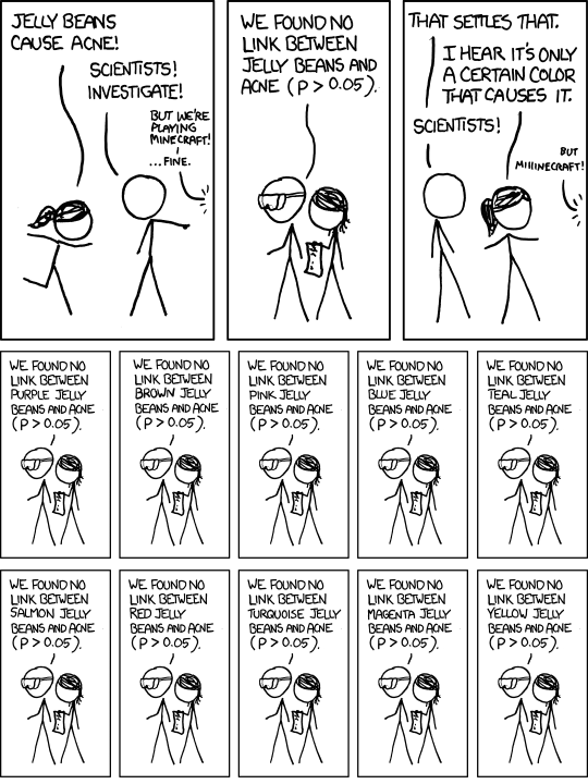
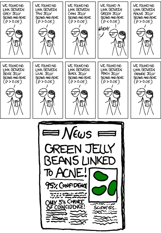
Jelly Beans and Acne
Suppose I have data on 1000 study participants. 500 of them are randomly assigned to eat no jelly beans for two months. The remaining 500 are split into 20 groups with 25 participants each. In each group, patients are assigned a particular color of jelly bean to consume. They eat 5 jelly beans a day of their assigned color over the course of two months. All 1000 participants count the total number of pimples they've had over the course of the study period.
-
What are the null hypotheses being tested in the xkcd strip?
-
What's my response variable?
-
What are my predictor variable(s)?
Jelly Beans and Acne
Suppose I have data on 1000 study participants. 500 of them are randomly assigned to eat no jelly beans for two months. The remaining 500 are split into 20 groups with 25 participants each. In each group, patients are assigned a particular color of jelly bean to consume. They eat 5 jelly beans a day of their assigned color over the course of two months. All 1000 participants count the total number of pimples they've had over the course of the study period.
-
How can I use multiple regression to assess the hypotheses under investigation?
-
What would be the underlying assumptions?
What Goes Wrong?
In general:
-
If we are conducting $K$ hypothesis tests, the probability of committing at least one type I error is bounded above by $K\alpha$ if each individual test is conducted at $\alpha$
A simple calculation assuming independence provides a bit more insight:
-
If we are testing $K$ null hypotheses that are actually true, and the hypothesis tests are independent from one another, the probability that we commit at least one type one error is exactly $1 - (1-\alpha)^K$.
-
At $\alpha = 0.05$, with $K=10$, this probability is 0.4.
-
At $K=20$, probability is 0.64
Familywise Error Rate
When conducting multiple hypothesis tests, the probability of committing at least one Type I error increases with the number of hypothesis tests we are considering
-
xkcd: separately testing whether purple, brown, pink, blue,... jelly beans have an effect, each using $\alpha=0.05$, results in a probability of committing at least one Type I error that is much larger than $0.05$!
When testing multiple hypotheses, we clearly need to make an adjustment to control this rate of false positives
Familywise Error Rate
Familywise Error Rate (FWER)
The Familywise Error Rate is the probability of rejecting at least one null hypothesis that is actually true when testing $K$ hypotheses. That is, it's the probability of committing at least one Type I error.
Often, we'll want to control the FWER at $\alpha_{family} = 0.05$.
The Bonferroni Correction
There's a simple way to correct for multiple comparisons and guarantee that the FWER is below a prespecified threshold regardless of the dependence between tests (sometimes test statistics are correlated — multiple regression is one example):
The Bonferroni Correction
If I conduct $K$ hypothesis tests, I can guarantee that the probability of committing at least one Type I error is at most $\alpha$ if I conduct each individual test at level $\alpha/K$
-
Example: if I conduct 5 tests, I can conduct each at level $0.05/5 = 0.01$ to guarantee probability of at least one Type I error is below 0.05.
Back to Jelly Beans...
In our simulation, we separately test whether $K=20$ colors of jelly beans caused acne. Employing the Bonferroni correction, if we want the family-wise error rate to be 0.05 we should conduct each individual test using $\alpha = 0.05/20$
reject.individ.bonf = (pval.individ <= 0.05/20)
reject.any.bonf = apply(reject.individ.bonf, 1, any)

> mean(reject.any.bonf)
[1] 0.0503
What's the Nature of the Differences?
The overall $\mathcal{F}$ test would provide us with a test of the null that, if I have $G$ categories for a categorical variable,
\begin{align*} \mathbf{H_o}: & \; \mu_{1} = \mu_{2} = \cdots = \mu_{G}\\ \mathbf{H_a}: & \; \text{at least one } \mu_i\neq \mu_j \end{align*}If we reject this null, we certainly might be interested in the precise nature of the differences.
-
Which groups are different?
-
In our medicorp example, do sales in the west differ from sales in the south?
What's the Nature of the Differences?
Explicitly, for any $i,j$, we might want to assess the null:
\begin{align*} \mathbf{H_o}: & \; \mu_{i} = \mu_{j}. \end{align*}Through using the Bonferroni correction, we are also entitled to talk about the individual results of all of comparisons we have made.
Bonferroni: Individual Conclusions
If I conduct $K$ hypotheses and use a Bonferroni correction, we are entitled to talk about the individual results of all of the $K$ comparisons we have made
-
If I rejected a null hypothesis even after applying a Bonferroni correction, I'd be allowed to say that the difference was statistically significant while accounting for the potential impact of multiple comparison
Contrast with the Overall $\mathcal{F}$ test:
-
Tells me something is going on...
-
...but doesn't let me talk about the particular nature of the differences. Doesn't tell me which particular slopes are nonzero.
The Cost of Multiple Comparisons
When using a Bonferroni correction when testing $K$ hypotheses, we reject the null when $p_{val} \leq \alpha/K$.
-
More stringent criterion controls the FWER. This is a good thing — reduces the likelihood of a spurious finding.
-
Unfortunately, more stringent criterion also makes it less likely that we'll correctly reject an incorrect null hypothesis
-
That is, the power of the resulting hypothesis test has been reduced.
-
In addition to reducing the risk of spurious/incorrect finding, it also reduces the chances of correct findings being flagged
The Cost of Multiple Comparisons
For this reason, there's a vast literature on methods besides Bonferroni for controlling for multiple comparisons.
-
Objective: control the FWER, while potentially providing improvements in power
Holm-Bonferroni
Despite its simplicity, it turns out there's a method that is uniformly better than Bonferroni known as Holm-Bonferroni. Order the $p$-values from my $K$ hypothesis tests as $p_{1} \leq p_2 \leq \cdots \leq p_K$:
-
Is $p_1 \leq \alpha/K$? If so, continue to the next step. Otherwise, stop.
-
If $p_1 \leq \alpha/K$, is $p_2 \leq \alpha/(K-1)$? If so, continue to the next step. Otherwise, stop.
-
In general, if the previous $i-1$ steps have been successful, in the $i$th step you test whether $p_i \leq \alpha/(K+1-i)$. Proceed if yes, stop otherwise.
Holm-Bonferroni
If the method terminates in step 1, we don't reject any null hypotheses. If it terminates in step $i$, you reject the hypotheses corresponding to $p_1,\ldots,p_{i-1}$. If it doesn't terminate, we reject all $K$ of our hypotheses.
-
Rejects as many or more hypotheses than Bonferroni, which compares all $p$-values to $\alpha/K$.
Tukey-Kramer HSD
Multiple regression with a single categorical predictor and no continuous predictors (like our jelly bean example) is sometimes referred to as "One-Way Analysis of Variance," or One-Way ANOVA.
-
Quite common in practice, for instance when assessing the effect of $G$ candidate interventions on an outcome of interest.
-
Large assumption when using ANOVA: equal variances across the groups being compared
In this context, there are particular methods built for comparing the average responses across different groups while controlling the FWER
Pairwise Comparisons
Suppose we have $G$ groups ($G$ levels of the categorical predictor). For all $i\neq j$, $i,j=1,\ldots,G$, we might want to assess the null:
\begin{align*} \mathbf{H_o}: & \; \mu_{i} = \mu_{j}. \end{align*}Suppose we want to make all $K=\binom{G}{2}$ possible pairwise comparisons between different groups, while controlling the FWER at level $\alpha$.
Example: $G=3$, we'd want to compare:
- $\mu_1$ to $\mu_2$
- $\mu_1$ to $\mu_3$
- $\mu_2$ to $\mu_3$.
Tukey-Kramer Honest Significant Difference
Let $\bar{y}_i$ be the observed mean in the $i$th of $G$ groups, and let $\widehat{\sigma}_\varepsilon$ be the RMSE from our regression of the response on the categorical predictor.
For all $i,j$, we can construct a $100(1-\alpha)\%$ confidence interval for $\mu_i-\mu_j$ while controlling the FWER at $\alpha$ through the following:
\begin{align*}\textstyle \bar{y}_i-\bar{y}_j \pm \frac{q_{1-\alpha, G, n-G}}{\sqrt{2}}\widehat{\sigma}_\varepsilon(\frac{1}{n_i} + \frac{1}{n_j})^{\frac12}, \end{align*}where $q_{1-\alpha, G, n-G}$ is a quantile from the Studentized Range Distribution, and $n_i$ is the sample size for the $i$th group.
-
Studentized Range $(G, n-G)$: Accounts for the fact that we are looking at $|\bar{y}_i-\bar{y}_j|$ for all possible combinations of groups.
-
Using it produces wider intervals than those from the $t$ distribution unless $G=2$
Medicorp: Tukey-Kramer CI
#Compare Studentized Range to t distribution
#w/o controlling for multiple comparisons
> qtukey(.95, 3, nrow(medicorp)-3)/sqrt(2)
[1] 2.504336
> qt(.975, nrow(medicorp)-3)
[1] 2.068658
> #Compute Tukey-Kramer CIs
> TukeyHSD(aov(Sales~Region, data = medicorp))

$Region
                   diff        lwr       upr     p adj
SOUTH-MIDWEST -461.0997 -642.69517 -279.5043 0.0000050
WEST-MIDWEST  -336.1042 -510.62592 -161.5825 0.0002066
WEST-SOUTH     124.9955  -69.39076  319.3818 0.2615627
Comparing Tukey to Bonferroni
For a given $G$, consider 95% confidence intervals in One-Way ANOVA.
-
Tukey-Kramer: $q_{0.95, G, n-G}/\sqrt{2}$
-
Bonferroni: $t_{1-0.025/K, n-G}$, where $K = \binom{G}{2}$.
How do these compare? Fix $n=1000$ for purpose of illustration:

Quantiles are the same for $G=2$. Tukey-Kramer is better (narrower CI) for $G>2$.
Pointwise Confidence Intervals
In regression, we've introduced methods for constructing 95% confidence intervals for $\mu_{y\mid \tilde{x}} = \text{E}(y \mid \tilde{x})$ at particular data points $\tilde{x}$.
-
These are called pointwise confidence intervals
-
For any particular point $\tilde{x}$, I am 95% confident that $\mu_{y\mid \tilde{x}}$ will fall within:
Suppose I construct these intervals at different points $\tilde{x}_1$, $\tilde{x}_2$,...,$\tilde{x}_K$. Am I still 95% confident that $\mu_{y\mid \tilde{x}_1}$,...,$\mu_{y\mid \tilde{x}_K}$ will all fall within those intervals?
Pointwise Confidence Intervals

At any particular point $\tilde{x}$, the dotted lines provide valid upper and lower bounds on a 95% confidence interval
However, this does not imply that we are 95% confident that the true prediction equation falls within these bounds. This would be making multiple comparisons!
Scheffé's Method
Rather than capturing $\mu_{y\mid \tilde{x}}$ at a given point $\tilde{x}$, can I create upper and lower bounds that capture the entire function $\text{E}(y\mid \tilde{x}) = \tilde{x}^\top\beta$ with $100(1-\alpha)\%$ confidence?
-
Seems daunting — requires comparisons at infinitely many points $\tilde{x}$!
-
Remarkably, the answer is yes, and the price is smaller than you might imagine.
Scheffé's Method
At any point $\tilde{x}$, consider the following modified confidence intervals for the conditional expectation:
\begin{align*} \widehat{\mu}_{y\mid \tilde{x}} \pm \sqrt{(p+1)\mathcal{F}_{1-\alpha,(p+1), n-p-1}}\;\widehat{\sigma}_\varepsilon \sqrt{\tilde{x}^\top(X^\top X)^{-1}\tilde{x}}, \end{align*}where $\mathcal{F}_{1-\alpha,(p+1), n-p-1}$ is the $1-\alpha$ quantile of an $\mathcal{F}$ distribution with $p+1$ and $n-p-1$ degrees of freedom.
Scheffé Correction
Replacing a quantile from the $t_{n-p-1}$ distribution with $\sqrt{(p+1)\mathcal{F}_{1-\alpha,(p+1), n-p-1}}$ is known as Scheffé's Correction
-
Accounts for looking at all possible linear combinations of $\widehat{\beta}$, all possible $\tilde{x}^\top\widehat{\beta}$
-
Size of penalty depends on the number of predictor variables.
-
In simple regression $(p=1)$, not so bad.
-
$p$ large, results in very wide intervals. Much wider than pointwise intervals.
The resulting intervals, when plotted for all values of $\tilde{x}$, capture the true prediction equation with $100(1-\alpha)\%$ confidence.
Simultaneous Confidence Bands
Purple bands are 95% simultaneous confidence bands for capturing the entire prediction equation.
