STATS 413: Lecture 13

Cook's distance
Multicollinearity
Partial regression
Variance inflation factor and condition number

Recap: Flagging Unusual Observations

From last class, we deemed a point an outlier if it "stood out" relative to the other observations in our data set.

Seems natural that outlying observations might have extreme values for their residuals. Why isn't this always the case?
What was leverage? Does it depend upon the distribution of the predictors or of the responses?
What observations have high leverage? Low leverage?
How did we overcome this when devising a test for whether or not an observation is an outlier?

Cook's Distance

The Cook's distance $D_i$ of an observation $i$ is the sum of the squared differences between predicted values in regressions fit including $i$ and excluding $i$, normalized by $(p+1)\hat{\sigma}_\varepsilon^2$

\begin{align*} D_i &= \frac{(X\widehat{\boldsymbol\beta} - X\widehat{\boldsymbol\beta}_{(i)})^\top(X\widehat{\boldsymbol\beta} - X\widehat{\boldsymbol\beta}_{(i)})}{(p+1)\hat{\sigma}^2_\varepsilon}, \end{align*}

where $\widehat{\boldsymbol\beta}_{(i)}$ are the regression coefficients from a regression excluding observation $i$.

Cook's Distance

Equivalently, Cook's distance can be expressed as

\begin{align*} D_i &= \frac{1}{p+1}r_i^2\frac{h_{ii}}{1-h_{ii}}, \end{align*}

from whence we see that $D_i$ combines the impact of

Large residual (in terms of standardized residual $r_i$)
Large leverage ($h_{ii}$)
Influence of a point on the OLS solution is a combination of these two attributes.

Rule of thumb: $D_i > 1$ indicates an influential point

Residuals vs Leverage

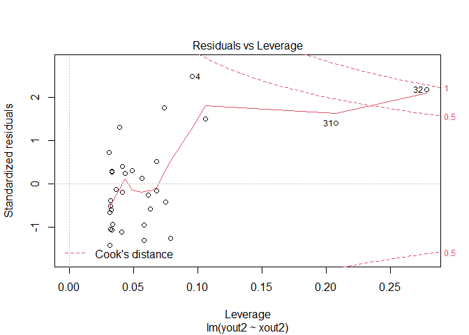
Contours correspond to values of Cook's Distance equal to 0.5 and 1. For instance, all points except 32 have a Cook's Distance less than 0.5. Point 32 is between 0.5 and 1.

Car Seat Position

Auto industry experts wanted to determine what features influence the positioning of the driver's seat for drivers. 38 volunteers were asked to sit in the driver's seat of a given car and adjust the positioning to their preference. Researchers recorded where the driver positioned the driver's seat.

Response: Hipcenter – measure of car seat position
Predictors: Age, Weight, various Height measurements (with shoes, without shoes, seated), arm, thigh, leg length.

Multiple Regression

            Estimate Std.Error t value Pr(>|t|)
(Intercept)436.43213 166.57162   2.620   0.0138
Age          0.77572   0.57033   1.360   0.1843
Weight       0.02631   0.33097   0.080   0.9372
HtShoes     -2.69241   9.75304  -0.276   0.7845
Ht           0.60134  10.12987   0.059   0.9531
Seated       0.53375   3.76189   0.142   0.8882
Arm         -1.32807   3.90020  -0.341   0.7359
Thigh       -1.14312   2.66002  -0.430   0.6706
Leg         -6.43905   4.71386  -1.366   0.1824

Residual standard error: 37.72 on 29 degrees of freedom
Multiple R-Squared: 0.6866   Adjusted R-squared: 0.6001
F-statistic:  7.94 on 8 and 29 DF    p-value: 1.306e-05

Compare the Overall $F$-tests to the individual $t$-tests on slope coefficients. Anything odd?

Multicollinearity

Multicollinearity/Collinearity refers to a situation where two or more predictor variables are strongly linearly related with one another.

\begin{align*} X &= \left ( \begin{array}{cccc} \vert & \vert & \cdots & \vert \\ 1 & x_1 & \cdots& x_p \\ \vert & \vert & \cdots & \vert \end{array} \right). \end{align*}

Multicollinearity

Perfect multicollinearity is rare: requires that one predictor variable $x_j$ can be expressed as a linear combination of the other predictors.

\begin{align*} x_j &= \alpha_0 + \alpha_1 x_1 +\dots + \alpha_{j-1}x_{j-1} + \alpha_{j+1}x_{j+1} + \dots + \alpha_px_p \end{align*}

Avoiding perfect multicollinearity came up when encoding categorical predictors as $G-1$ dummy variables.

More frequently, our concern is with strong, not perfect, collinearity.

\begin{align*} x_j &\approx \alpha_0 + \alpha_1x_1 \dots + \alpha_{j-1}x_{j-1} + \alpha_{j+1}x_{j+1} + \dots + \alpha_px_p \end{align*}

Multicollinearity vs Leverage

Both multicollinearity and leverage have to do with the distribution of the predictors, versus the responses.

They describe very different attributes of predictor space, with different statistical ramifications

Leverage: certain observations are outliers with respect to the distribution of $X$. Have potential to exert large influence over the OLS solution
Multicollinearity: Predictor space is nearly degenerate. Any predictor $x_i$ "nearly" resides in a lower-dimensional subspace of $\mathbb{R}^p$.

Consequences of Collinearity

Mathematical issue: $X^\top X$ close to singular (i.e. $X^\top X$ close to being non-invertible).

If $X^\top X$ is close to singular, $(X^\top X)^{-1}$ large and unstable

Small changes in $X$ can have a large impact on $(X^\top X)^{-1}$
Think of this in analogy to $1/|\delta|$ when $\delta$ is nearly zero. Small change in $\delta$, big change in $1/|\delta|$

Consequences of Collinearity

Recall that

\begin{align*} \widehat{\boldsymbol\beta} = (X^\top X)^{-1}X^\top y \end{align*}

Because $\widehat{\boldsymbol\beta}$ depends on $(X^\top X)^{-1}$, collinearity has many statistical ramifications:

Imprecise / unstable estimates of $\beta$
Strong sensitivity of $\widehat{\boldsymbol\beta}$ to rounding of predictor variables, or slight measurement errors.
$t$-tests can fail to reveal significant predictors

Consequences of Collinearity

Recall that

\begin{align*} \widehat{\boldsymbol\beta} = (X^\top X)^{-1}X^\top y \end{align*}

Because $\widehat{\boldsymbol\beta}$ depends on $(X^\top X)^{-1}$, collinearity has many statistical ramifications:

Coefficients can have "weird" signs and values relative to our intuition
Estimated prediction equation, $\tilde{x}^\top\widehat{\boldsymbol\beta}$, highly unstable.
- Slight change in $X$, big change in my predictions for $y$ at a future observation $\tilde{x}$.

Diagnosing Collinearity: A 1st Attempt

A first place to start is investigating:

Pairwise Scatterplots
Pairwise Correlations

Looking for any extremely strong (say, $>0.9$) correlations

> cor(predictors)
               income competitors  visitors
income      1.0000000   0.4021462 0.4937368
competitors 0.4021462   1.0000000 0.6973704
visitors    0.4937368   0.6973704 1.0000000

> pairs(predictors)

Limitations of Pairwise Correlations

Pairwise correlations and scatterplots help us assess if any pairs of predictor variables are strongly related.

Issue: What if one predictor is (nearly) a linear combination of multiple predictor variables?

Pairwise scatterplots and correlations won't reveal this

To devise a metric for assessing multicollinearity more generally, we'll now dive into the role that multicollinearity plays in determining $\widehat{\beta}_j$ and its standard error.

Another way of Computing $\widehat{\beta}_j$

To calculate the $j$th estimated slope coefficient $\widehat{\beta}_j$, we use the $j+1$st coordinate of

\begin{align*} \widehat{\boldsymbol\beta} &= (X^\top X)^{-1}X^\top y \end{align*}

We'll now illustrate a different approach. To do this, let $X_{R}$ be a $n\times p$ matrix containing all of the predictor variables except the $j$th predictor (the "rest" of the predictor variables besides $j$).

Another way of Computing $\widehat{\beta}_j$

\begin{align*} X_{R} &= \left ( \begin{array}{ccccccc} \vert & \vert & \cdots & \vert&\vert& \cdots& \vert \\ 1 & x_1 & \cdots& x_{j-1} & x_{j+1}&\cdots& x_p \\ \vert & \vert & \cdots & \vert &\vert&\cdots&\vert \end{array} \right). \end{align*}

Let $H_{R}$ be the hat matrix corresponding to $X_{R}$:

\begin{align*} H_{R} &= X_{R}(X_{R}^\top X_{R})^{-1}X_{R}^\top \end{align*}

Partial Regression

Consider running the following two regressions:

$y$ on $X_{R}$
$x_j$ on $X_{R}$

Define the residuals from these regressions as

\begin{align*} y_{.R} &= (I-H_R)y\\ x_{j.R} &= (I-H_R)x_j \end{align*}

Partial Regression

Now, consider running a simple regression of $y_{.R}$ on $x_{j.R}$.

$y_{.R}$ is the component of $y$ that cannot be explained as a linear function of the covariates $X_R$. It is $y$ adjusted for $X_R$.
$x_{j.R}$ is the component of $x_j$ that cannot be explained as a linear function of the covariates $X_R$. It is $x_j$ adjusted for $X_R$.

Partial Regression

Note that $\bar{y}_{.R}=\bar{x}_{j.R}=0$ (why? they are averages of residuals from regressions including an intercept term). Therefore:

\begin{align*} \widehat{\beta}_{0.R} &= 0\\ \widehat{\beta}_{j.R} &= \frac{\sum_{i=1}^N x_{ij.R}y_{i.R}}{\sum_{i=1}^n x_{ij.R}^2}\\ &= \frac{x_j^\top(I-H_R)y}{x_{j}^\top(I-H_R)x_j} \end{align*}

Partial Regression

Again letting $\widehat{\beta}_j$ be the $j+1$ coordinate of $\widehat{\boldsymbol\beta} = (X^\top X)^{-1}X^\top y$:

Multiple Regression Slopes Through Partial Regression

\begin{align*} \widehat{\beta}_{j.R} &= \widehat{\beta}_j \end{align*}

See the end of the notes for a (optional, you won't be tested on it) proof.

Partial Regression

Conclusion: in a regression of $y_{.R}$ on $x_{j.R}$

Intercept equals zero
Slope equals $\widehat{\beta}_j$
Residuals are identical to the residuals in a regression of $y$ on $X$ (weird!).

Partial Regression

Note: a scatter plot of $y_{.R}$ against $x_{j.R}$ is called a partial regression plot. Can be used as an additional diagnostic tool to detect:

Nonlinearity
Heteroskedasticity
Influential points for determining the $j$th slope coefficient

We won't dwell on this further here, but you may see partial regression plots in practice.

An Equivalent Form for $\text{var}(\widehat{\beta}_j)$

Because $\widehat{\beta}_j = \widehat{\beta}_{j.R}$, it must be the case that

\begin{align*} \text{var}(\widehat{\beta}_j) &= \text{var}(\widehat{\beta}_{j.R}) \end{align*}

Let's use the form of $\widehat{\beta}_{j.R}$ to derive another expression for $\text{var}(\widehat{\beta}_j) = \sigma^2_\varepsilon(X^\top X)^{-1}_{(j+1),(j+1)}$

The Variance of $\widehat{\beta}_j$

\begin{align*} \text{Var}(\widehat{\beta}_j) &= \frac{\sigma^2_\varepsilon}{x_j^\top(I-H_R)x_j}\\ &= \frac{\sigma^2_\varepsilon}{\sum_{j=1}^n x_{ij.R}^2} \end{align*}

Connections with Multicollinearity

This result provides another (equivalent) way to compute standard errors:

\begin{align*} \text{se}(\widehat{\beta}_j) &= \frac{\hat{\sigma}_\varepsilon}{\sqrt{x_j^\top(I-H_R)x_j}} \end{align*}

That said, the main reason we've gone through partial regression is that it inspires a useful measure of multicollinearity.

Measure how "unstable" a slope coefficient is because of multicollinearity.
Instability = High variance

Connections with Multicollinearity

This result provides another (equivalent) way to compute standard errors:

\begin{align*} \text{se}(\widehat{\beta}_j) &= \frac{\hat{\sigma}_\varepsilon}{\sqrt{x_j^\top(I-H_R)x_j}} \end{align*}

That said, the main reason we've gone through partial regression is that it inspires a useful measure of multicollinearity.

How much has the variability in the slope coefficient increased due to multicollinearity?
This metric will be based, in part, on the term under the square root

\[ x_j^\top(I-H_R)x_j \]

$SSE$ for Predictors

We can think of $x_j^\top(I-H_R)x_j$ as a type of $SSE$ from our partial regression framework

\begin{align*} SSE_j &= x_j^\top(I-H_R)x_j = \sum_{i=1}^n (x_{ij} - \hat{x}_{ij})^2, \end{align*}

where $\hat{x}_{ij}$ are my predicted values from a regression of $x_{ij}$ on $X_R$

$SST$ for Predictors

The corresponding $SST$ for this partial regression is

\begin{align*} SST_j &= \sum_{i=1}^n(x_{ij} - \bar{x}_j)^2 = (n-1)\text{var}(x_j), \end{align*}

where $\text{var}(x_j)$ is the sample variance.

Generally, we prefer $SSE$ to be small relative to $SST$
In this context however, $SSE_j$ small relative to $SST_j$ indicates strong multicollinearity!
It means we can predict $x_j$ very well as a linear function of the other predictor variables.

No Multicollinearity: Orthogonality

There would be no multicollinearity issues with respect to $x_j$ and $\widehat{\beta}_j$ if

\begin{align*} SSE_j &= SST_j \end{align*}

When would this occur?

If $\frac{1}{n}\sum_{i=1}^n(x_{ij}-\bar{x}_j)(x_{ik}-\bar{x}_k) = 0$ for $k=1,..,p$; $k\neq j$.
That is, if $x_j$ minus its sample mean orthogonal to the other $p-1$ predictor variables minus their sample means.

No Multicollinearity: Orthogonality

If $x_j - \bar{x}_j$ orthogonal to $x_k - \bar{x}_k$ for $k=1,...,p$, $k\neq j$:

\begin{align*} x_{ij.R} &= x_{ij} - \bar{x}_j \end{align*}

In this case, the following two slopes are identical:

The estimated slope coefficient on $x_j$ in a simple regression of $y$ on $x_j$
The estimated slope coefficient on $x_j$ in a multiple regression of $y$ on $x_1$,$x_2$,...,$x_p$.

Orthogonality and Estimated Slope Coefficients

If $x_j$, centered by its mean, is orthogonal to $x_k$, centered by its mean, for $k=1,...,p$, $k\neq j$, the slopes on $\widehat{\beta}_j$ in simple and multiple regression are the same!

Compare our interpretations of the slope on $\widehat{\beta}_j$ in simple and multiple regression

Simple regression: Two individuals who differ in $x_j$ by one unit are estimated to differ in $y$ by $\widehat{\beta}_j$
Multiple regression: Holding the values for the other predictor variables fixed, two individuals who differ in $x_j$ by one unit are estimated to differ in $y$ by $\widehat{\beta}_j$

Orthogonality and Estimated Slope Coefficients

Under orthogonality, these two estimates are the same.

Adjusting for other predictors does nothing to alter the impact of differences in $x_j$ on differences in $y$.
None of the other predictors systematically vary with $x_j$.

Comparing Actual Variance to Ideal Variance

Using this new $SSE$ notation,

\begin{align*} \text{Var}(\widehat{\beta}_j) &= \frac{\sigma^2_\varepsilon}{SSE_j} \end{align*}

From this, we see that the smallest variance for $\widehat{\beta}_j$ is attained when $SSE_j = SST_j$

Smallest variance = most stable estimate (no multicollinearity)

Comparing Actual Variance to Ideal Variance

Comparing to this ideal:

\begin{align*} \text{Var}(\widehat{\beta}_j) &= \frac{\sigma^2_\varepsilon}{SST_j}\frac{SST_j}{SSE_j}\\ &= \left(\frac{\sigma^2_\varepsilon}{SST_j}\right)\left(\frac{1}{1-R^2_j}\right), \end{align*}

where $R^2_j = 1-SSE_j/SST_j$

Variance Inflation Factor

The Variance Inflation Factor (VIF) for covariate $j$ is defined to be

\begin{align*} VIF_j &= \left(\frac{1}{1-R^2_j}\right), \end{align*}

where $R^2_j$ is the $R^2$ value from a regression of $x_j$ on the other predictor variables, $X_R$.

Answers question: "by what factor is the variance of $\widehat{\beta}_j$ inflated relative to what it would have been under no multicollinearity (orthogonality)."

Larger inflation – more unstable, higher impact of multicollinearity.
Rule of thumb, $VIF_j>10$ concerning (some use $VIF_j>5$ as threshold).

The Condition Number

Another metric for multicollinearity will be based on the condition number for the correlation matrix of the predictors. Consider a system of equations of the form

\begin{align*} Ab = c \end{align*}

Condition number of $A$ is a derivative of sorts.

The condition number of $A$ answers the question: "how quickly does $b$ change due to a small change in $c$?"

The Condition Number

In linear regression, we consider the normal equations:

\begin{align*} (X^\top X)\widehat{\boldsymbol\beta} & = X^\top y \end{align*}

How rapidly does $\widehat{\boldsymbol\beta}$ change with a small change in $X^\top y$? A measure of instability...

Condition Number of Correlation Matrix

The condition number of $(X^\top X)$ itself depends upon the units of $X$, making it inappropriate as a measure of multicollinearity

We instead consider the condition number of the correlation matrix for the predictor variables.

Correlations – invariant to changes in units, and contain the necessary information about multicollinearity
The correlation matrix $C$ has entries $C_{ij} = \text{cor}(x_i, x_j)$

Condition Number of Correlation Matrix

The condition number $\kappa$ is defined to be

\begin{align*} \kappa &= \sqrt{\frac{\lambda_{1}}{\lambda_{p}}}, \end{align*}

where $\lambda_{1}$ and $\lambda_{p}$ are the largest and smallest eigenvalues of the correlation matrix for the predictors. Rules of thumb: $\kappa > 15$ indicates moderate collinearity; $\kappa > 30$ indicates big issues.

Return to Seatbelt Example

Car drivers adjust the seat position for comfort
Response: seat position
Predictors: age, weight, height with and without shoes, seated height, arm length, thigh length, lower leg length

Regression Results

            Estimate Std.Error t value Pr(>|t|)
(Intercept)436.43213 166.57162   2.620   0.0138
Age          0.77572   0.57033   1.360   0.1843
Weight       0.02631   0.33097   0.080   0.9372
HtShoes     -2.69241   9.75304  -0.276   0.7845
Ht           0.60134  10.12987   0.059   0.9531
Seated       0.53375   3.76189   0.142   0.8882
Arm         -1.32807   3.90020  -0.341   0.7359
Thigh       -1.14312   2.66002  -0.430   0.6706
Leg         -6.43905   4.71386  -1.366   0.1824

Residual standard error: 37.72 on 29 degrees of freedom
Multiple R-Squared: 0.6866   Adjusted R-squared: 0.6001
F-statistic:  7.94 on 8 and 29 DF    p-value: 1.306e-05

Sensitivity of Coefficients to Perturbations of $y$

> junk <- lm(hipcenter + 10*rnorm(38) ~ ., data=seatpos)

            Estimate Std.Error t value Pr(>|t|)
(Intercept)431.13413 176.13709   2.448   0.0207
Age          0.60041   0.60308   0.996   0.3277
Weight      -0.10886   0.34998  -0.311   0.7580
HtShoes     -3.86967  10.31311  -0.375   0.7102
Ht           1.33472  10.71159   0.125   0.9017
Seated       0.79736   3.97792   0.200   0.8425
Arm         -0.01702   4.12417  -0.004   0.9967
Thigh       -1.54993   2.81278  -0.551   0.5858
Leg         -4.73289   4.98456  -0.950   0.3502

Residual standard error: 39.89 on 29 degrees of freedom
Multiple R-Squared: 0.656    Adjusted R-squared: 0.5611
F-statistic: 6.912 on 8 and 29 DF    p-value: 4.451e-05

Detection of Collinearity

Correlation matrix: large pairwise correlation
Regress $x_j$ on other predictors $\Rightarrow$ $R_j^2$. $R_j^2$ above 0.9 indicates a problem. Equivalently, check if $VIF_j > 10$.
Condition number of correlation matrix: $\kappa = \sqrt{\frac{\lambda_1}{\lambda_{p}}}$ (for checking numerical stability)

Overall Correlation Matrix

## Correlation matrix
> round(cor(seatpos[,1:8]), 2)
          Age Weight HtShoes    Ht Seated  Arm Thigh   Leg
Age      1.00   0.08   -0.08 -0.09  -0.17 0.36  0.09 -0.04
Weight   0.08   1.00    0.83  0.83   0.78 0.70  0.57  0.78
HtShoes -0.08   0.83    1.00  1.00   0.93 0.75  0.72  0.91
Ht      -0.09   0.83    1.00  1.00   0.93 0.75  0.73  0.91
Seated  -0.17   0.78    0.93  0.93   1.00 0.63  0.61  0.81
Arm      0.36   0.70    0.75  0.75   0.63 1.00  0.67  0.75
Thigh    0.09   0.57    0.72  0.73   0.61 0.67  1.00  0.65
Leg     -0.04   0.78    0.91  0.91   0.81 0.75  0.65  1.00

Explaining Insignificance

$p$-value on covariate $j$ assesses whether or not, after having included the other $p-1$ predictor variables in the model, we also need to include covariate $j$.

Under stronger multicollinearity, the other $p-1$ predictor variables contain substantial information about $j$ due to strong correlations
So, in a sense, by including the other $p-1$ variables we have also more or less included covariate $j$ if there's a collinearity issue
For instance, Ht insignificant: we had already included HtShoes and Seated. After including those variables, Ht itself didn't bring much additional to the table.

Condition Number of Correlation Matrix

## Condition number
eigs.seat = eigen(cor(seatpos[,1:8]))$values
condnumber = sqrt(eigs.seat[1]/eigs.seat[length(eigs.seat)])
condnumber
[1] 59.7662

Variance Inflation Factors

## Variance inflation factor
> library(faraway)
> vif(lm.seat)
       Age     Weight    HtShoes         Ht     Seated
  1.997931   3.647030 307.429378 333.137832   8.951054
       Arm      Thigh        Leg
  4.496368   2.762886   6.694291

Correlations of Length Measurements

## Correlation of variables measuring length
> round(cor(seatpos[,3:8]),2)
        HtShoes   Ht Seated  Arm Thigh  Leg
HtShoes    1.00 1.00   0.93 0.75  0.72 0.91
Ht         1.00 1.00   0.93 0.75  0.73 0.91
Seated     0.93 0.93   1.00 0.63  0.61 0.81
Arm        0.75 0.75   0.63 1.00  0.67 0.75
Thigh      0.72 0.73   0.61 0.67  1.00 0.65
Leg        0.91 0.91   0.81 0.75  0.65 1.00

Using a Subset of Predictor Variables

## Using a subset of predictor variables
> result2 <- lm(hipcenter ~ Age + Weight + Ht, data=seatpos)
> summary(result2)
Coefficients:
            Estimate Std.Error t value Pr(>|t|)
Intercept 528.297729 135.31295   3.904 0.000426
Age         0.519504  0.408039   1.273 0.211593
Weight      0.004271  0.311720   0.014 0.989149
Ht         -4.211905  0.999056  -4.216 0.000174

Residual standard error: 36.49 on 34 degrees of freedom
Multiple R-Squared: 0.6562   Adjusted R-squared: 0.6258
F-statistic: 21.63 on 3 and 34 DF    p-value: 5.125e-08

What to Do about Multicollinearity?

If you mostly care about prediction accuracy for future observations, you should eliminate predictors that are highly correlated with other predictors.
Collinearity makes the prediction equation unstable! Substantially different prediction equations can fit the observed data similarly. Small changes in $X$ can yield big changes in predictions for new observations.

What to Do about Multicollinearity?

Try to use problem-specific context to choose which collinear variables to eliminate. That said, there are automated methods for variable selection which we will discuss soon
If interpretation is important and you must keep all predictors, be forewarned that coefficient estimates will be unstable. May be advisable to not use ordinary least squares, and to instead use a more advanced regression technique (stay tuned).

Optional: Proof of Partial Regression Result

Start with the decomposition

\begin{align*} y &= X\widehat{\boldsymbol\beta} + e\\ y &= X\widehat{\boldsymbol\beta} + (I-H)y, \end{align*}

where $H$ is the hat matrix based upon all of $X$. Multiply the second line by $(I-H_R)$

\begin{align*} (I-H_R)y &= (I-H_R)X\widehat{\boldsymbol\beta} + (I-H_R)(I-H)y \end{align*}

Observe that

\begin{align*} (I-H_R)X_R &= 0\\ (I-H_R)(I-H)&= (I-H) \end{align*}

Both of these stem from $X_R$ residing in the columnspace of $X$, so that $X_R H = X_R$ and $H_R H = H_R$.

Optional: Proof of Partial Regression Result

$(I-H_R)y = (I-H_R)X\widehat{\boldsymbol\beta} + (I-H_R)(I-H)y$ can be expressed as

\begin{align*} y_{.R} &= x_{j.R}\widehat{\beta}_j + (I-H)y. \end{align*}

Subtract $x_{j.R}\widehat{\beta}_j$ from both sides, and multiply by $x_j^\top(I-H_R)$

\begin{align*} x_{j.R}^\top(y_{.R} - x_{j.R}\widehat{\beta}_j) &= x_{j}^\top(I-H_R)(I-H)y \end{align*}

Remembering that $x_j$ is in the columnspace of $X$ and that $(I-H_R)(I-H) = (I-H)$, the right-hand side equals zero, as $x_j^\top(I-H)y = 0$.

Implication:

$\widehat{\beta}_j$ satisfies the normal equations for a regression of $y_{.R}$ on $x_{j.R}$
Of course, so too does $\widehat{\beta}_{j.R}$ (it comes from directly running the regression).
Solution is unique, so they must be the same!