STATS 413: Lecture 10
-
Inference for the regression function
-
Prediction intervals
Recap: Linear Combinations
Suppose I want to test the null that the difference in slope coefficients on Advertising between the south and the west equals zero, against the alternative that it is not zero. Test at $\alpha=0.05$
                    Estimate Std. Error t value Pr(>|t|)
(Intercept)        -555.5274   212.5735  -2.613  0.01817 *
RegionSOUTH         837.0791   292.4465   2.862  0.01079 *
RegionWEST          527.3892   393.8955   1.339  0.19823
Bonus                 1.8994     0.6424   2.957  0.00883 **
Advert                2.6585     0.2132  12.469 5.59e-10 ***
RegionSOUTH:Bonus    -0.8742     0.9571  -0.913  0.37382
RegionWEST:Bonus      0.7477     1.0145   0.737  0.47117
RegionSOUTH:Advert   -1.5546     0.4800  -3.239  0.00483 **
RegionWEST:Advert -1.6964 0.5644 -3.006 0.00796 **-
What's my estimate for this difference?
-
Can I calculate the standard error using this output?
Recap: Linear Combinations
-
Define a vector $a = (a_1,...,a_9)^\top$ such that \begin{align*} a^\top\hat{\beta} &= \hat{\beta}_\text{Advert, South} - \hat{\beta}_\text{Advert, West} \end{align*}
-
How can I use this result to calculate a standard error for $\hat{\beta}_\text{Advert, South} - \hat{\beta}_\text{Advert, West}$?
-
What would my test statistic look like?
-
How could I redefine the "reference category" in order to conduct this test without resorting to our results on linear combinations of slopes?
 [1,] "(Intercept)"
 [2,] "RegionSOUTH"
 [3,] "RegionWEST"
 [4,] "Bonus"
 [5,] "Advert"
 [6,] "RegionSOUTH:Bonus"
 [7,] "RegionWEST:Bonus"
 [8,] "RegionSOUTH:Advert"
 [9,] "RegionWEST:Advert"
Mall Sales
A retail company selling women's clothing has franchises across malls in America. It wants to investigate which factors are predictive of the number of sales per square foot of floor space (to level the playing field, since stores have varying footprints), and has collected annual data on $n=64$ of its stores. The company has a host of variables which it thinks may be predictive of sales. Two which we'll investigate:
-
Median income of the surrounding community (in thousands of dollars).
-
Number of competitor stores within the mall.
Regression Output
            Estimate Std. Error t value Pr(>|t|)
(Intercept)  91.4221    53.2652   1.716 0.091172 .
competitors -25.1345     6.3667  -3.948 0.000207 ***
income        7.4951     0.8909   8.413  8.6e-12 ***
Residual standard error: 67.42 on 61 degrees of freedom
Multiple R-squared:  0.5384, Adjusted R-squared:  0.5233
F-statistic: 35.58 on 2 and 61 DF,  p-value: 5.748e-11
Make sure you understand everything shown in this table, except for Adjusted R-squared (more on that later in the course)
- Prediction equation
- Hypothesis tests for individual slope coefficients
- Overall $\mathcal{F}$-test
- Degrees of freedom
- Residual standard error ($\hat{\sigma}_\varepsilon$)
- Multiple R-squared ($R^2$)
The Distribution of $\hat{\mu}_{y\mid \tilde{x}}$
To understand the distribution of $\hat{\mu}_{y\mid\tilde{x}} = \tilde{x}^\top\hat{\beta}$, let's use our results on linear combinations of slopes:
\begin{align*} E(\hat{\mu}_{y\mid\tilde{x}}) &= \mu_{y\mid \tilde{x}}\\ \text{var}(\hat{\mu}_{y\mid\tilde{x}}) &= \sigma^2_\varepsilon \tilde{x}^\top(X^\top X)^{-1}\tilde{x}\\ \hat{\mu}_{y\mid\tilde{x}} &\sim N(\mu_{y\mid \tilde{x}},\sigma^2_\varepsilon \tilde{x}^\top(X^\top X)^{-1}\tilde{x}) \end{align*}We can further estimate $\text{sd}(\hat{\mu}_{y\mid \tilde{x}})$ using the following standard error:
\begin{align*} \text{se}(\hat{\mu}_{y\mid \tilde{x}}) &= \hat{\sigma}_\varepsilon \sqrt{\tilde{x}^\top(X^\top X)^{-1}\tilde{x}} \end{align*}The Variability of $\hat{\mu}_{y\mid \tilde{x}}$
We see that $\text{se}(\hat{\mu}_{y\mid \tilde{x}}) = \hat{\sigma}_\varepsilon \sqrt{\tilde{x}^\top(X^\top X)^{-1}\tilde{x}}$ depends on the value of $\tilde{x}$.
-
What values of $\tilde{x}$ yield smaller variability? Larger variability?
The answer:
- Smallest variability: $\tilde{x} = (1, \bar{x}_1,\ldots,\bar{x}_p)$, the mean of the predictor variables
- Variability increases as $\tilde{x}$ moves farther from the mean.
Accords with intuition
- More information about what's occurring near the center of my data
- Less information in the extremes
The variability of $\hat{\mu}_{y\mid \tilde{x}}$
Through a bit of linear algebra (no need to derive), we can get an alternative form that makes this clear
-
Let $H_0$ be the "hat" matrix from a regression including only the intercept column.
-
Let $X_1$ be our design matrix without the intercept column (so it has $p$ columns, one for each predictor, and $n$ rows)
-
Let $\tilde{a}_1 = (\tilde{x}_1,\ldots,\tilde{x}_p)^\top$ be the point of interest, with the intercept entry excluded
-
Let $\bar{a}_1 = (\bar{x}_1,\ldots,\bar{x}_p)^\top$ be the means of the predictor variables in our data
The variability of $\hat{\mu}_{y\mid \tilde{x}}$
\begin{align*} \text{se}(\hat{\mu}_{y\mid \tilde{x}}) = \hat{\sigma}_\varepsilon \sqrt{\frac{1}{n} + (\tilde{a}_1 - \bar{a}_1)^ \top(X_1^\top(I-H_0)X_1)^{-1}(\tilde{a}_1 - \bar{a}_1)} \end{align*}Second term under square root is always non-negative
-
If $\tilde{a}_1 = \bar{a}_1$, second term cancels out, left with $\hat{\sigma}_\varepsilon/\sqrt{n}$
OLS Prediction Eq Passes Through the Mean
A consequence of the normal equations is that the OLS solution always passes through the point $(\bar{x}_1,\bar{x}_2,\ldots,\bar{x}_p, \bar{y})$.
-
Normal equations: $X^\top(X\hat{\beta}) = X^\top y$
The first normal equation takes the form:
\begin{align*} \hat{\beta}_0 n + \hat{\beta}_1\sum_{i=1}^nx_{i1} + \ldots + \hat{\beta}_p\sum_{i=1}^nx_{ip} &= \sum_{i=1}^n y_i \end{align*}OLS Prediction Eq Passes Through the Mean
Dividing by $n$...
\begin{align*} \hat{\beta}_0 + \hat{\beta}_1\bar{x}_1 + \ldots + \hat{\beta}_p\bar{x}_p &= \bar{y} \end{align*}So, when setting $\tilde{x} = (1, \bar{x}_1,\ldots,\bar{x}_p)$:
-
Estimate of $E(Y\mid x = \tilde{x})$ is $\hat{\mu}_{y\mid \tilde{x}} = \bar{y}$
-
Standard error of estimate is $\hat{\sigma}_{\varepsilon}/\sqrt{n}$
Inference for Conditional Expectation
Suppose the stronger linear model holds. A $100(1-\alpha)\%$ $t$-based confidence interval for ${\mu}_{y\mid \tilde{x}}$ is:
\begin{align*} \hat{\mu}_{y\mid \tilde{x}} \pm t_{1-\alpha/2, n-p-1}\text{se}(\hat{\mu}_{y\mid \tilde{x}}) \end{align*}-
Intervals are centered at the prediction from our estimated regression line, $\hat{\mu}_{y\mid \tilde{x}} = \tilde{x}^\top\hat{\beta}$.
Likewise, under the stronger linear model, we could form a test statistic to test the null $H_0: {\mu}_{y\mid \tilde{x}} = \mu_0$ of the form
\begin{align*} t_{stat} &= \frac{\hat{\mu}_{y\mid \tilde{x}} - \mu_0}{\text{se}(\hat{\mu}_{y\mid \tilde{x}})}, \end{align*}and compute $p$-values using a $t_{n-p-1}$ distribution.
Confidence Intervals in R
The intervals tend to be more popular in practice than the tests. R can create the intervals
within the predict command if we ask for them...
> lm.fatherson = lm(Son.Height~Father.Height,
data = fatherson)
> newfather = data.frame(Father.Height = 76)
> predict(lm.fatherson, newdata = newfather,
interval = "confidence", level = 0.95)
       fit      lwr      upr
1 74.49751 74.03653 74.95849
fit is the prediction from the regression line. lwr and upr are the
lower and upper bounds of the 95% Confidence Interval.
A Visualization

Displayed are the 95% confidence intervals plotted as a function of Father's height. Note that the OLS prediction equation forms the center of the intervals, and they are narrowest at the mean of father's height.
A Hypothesis Test
\begin{align*} \hat{\mu}_{y\mid \tilde{x}} &= 27.5253 + 0.6181\times \tilde{x}_1 \end{align*}At $\alpha=0.05$, is there evidence that sons whose fathers are 74 inches tall are shorter than 74 inches, on average?
> predict(lm.fatherson, newdata =
data.frame(Father.Height = 74), se=T)
$fit
      1
73.2614
$se.fit
[1] 0.1696489
$df
[1] 393Reject the null, suggest that average height for these sons is below 74 inches.
Future Predictions
I'm interested in opening a store in a new mall, where there are:
- 3 competitors
- The median income was 75K
First, using our regression equation, what's our prediction for the sales per square foot in the new location?
\begin{align*} \hat{\mu}_{y\mid \tilde{x}} = \tilde{x}^\top\hat{\beta},\quad\tilde{x} = (1,75,3)^\top \end{align*}xnew = data.frame(income = 75, competitors = 3)
predict(lm.both, newdata = xnew)
1
578.1509Do we think this prediction will be perfect? Or would we expect actual sales to differ from our prediction?
Motivating Prediction Intervals
Motivation: We know our predicted values $\hat{y}$ are just compromises, best guesses, linear approximations....
-
There's still left over variability that we can't account for
-
In our data: $R^2$ won't equal 1; residuals $e_i$ won't equal zero.
-
If we just give someone a prediction, we give them no sense of how much uncertainty is left over!
Motivating Prediction Intervals
-
Predicting sales will be 600 with an uncertainty range of $[580, 620]$ is much different than predicting sales will be 600 with a range of $[400, 800]$
-
Why not form an interval around my prediction that has a promise of catching future observations $y^*$ at a particular $\tilde{x}$ value 95% of the time?
-
These will be called prediction intervals
Recap: Inference for Conditional Expectations
Suppose $y_1,...,y_n$ are generated from the (stronger) linear model:
\begin{align*} y_i &= \beta_0 + \beta_1x_{i1} + ... + \beta_px_{ip} + \varepsilon_i,\\ \varepsilon_i &\overset{iid}{\sim}N(0, \sigma^2_\varepsilon). \end{align*}For any particular value for the predictors $\tilde{x} = (1, \tilde{x}_1,...,\tilde{x}_p)^\top$:
\begin{align*} \mu_{y\mid \tilde{x}} = E(y\mid x = \tilde{x}) &= \beta_0 + \beta_1\tilde{x}_{1} + ... + \beta_p\tilde{x}_{p}\\ &= \tilde{x}^\top\beta \end{align*}After running OLS regression and obtaining my estimate $\hat{\beta}$:
\begin{align*} \hat{\mu}_{y\mid \tilde{x}} = \hat{E}(y\mid x = \tilde{x}) &= \hat{\beta}_0 + \hat{\beta}_1\tilde{x}_{1} + ... + \hat{\beta}_p\tilde{x}_{p}\\ &= \tilde{x}^\top\hat{\beta} \end{align*}Recap: Inference for Conditional Expectations
A $100(1-\alpha)\%$ $t$-based confidence interval for ${\mu}_{y\mid \tilde{x}}$ is:
\begin{align*} \hat{\mu}_{y\mid \tilde{x}} &\pm t_{1-\alpha/2, n-p-1}\text{se}(\hat{\mu}_{y\mid \tilde{x}});\\ \text{se}(\hat{\mu}_{y\mid \tilde{x}}) &= \hat{\sigma}_\varepsilon\sqrt{\tilde{x}^\top(X^\top X)^{-1}\tilde{x}} \end{align*}
-
Centered at $\hat{\mu}_{y\mid \tilde{x}} = \tilde{x}^\top\hat{\beta}$.
-
Narrowest at mean of covariates
-
Wider at the extremes
Recap: Inference for Conditional Expectations
A $100(1-\alpha)\%$ $t$-based confidence interval for ${\mu}_{y\mid \tilde{x}}$ is:
\begin{align*} \hat{\mu}_{y\mid \tilde{x}} &\pm t_{1-\alpha/2, n-p-1}\text{se}(\hat{\mu}_{y\mid \tilde{x}});\\ \text{se}(\hat{\mu}_{y\mid \tilde{x}}) &= \hat{\sigma}_\varepsilon\sqrt{\tilde{x}^\top(X^\top X)^{-1}\tilde{x}} \end{align*}Is the above confidence interval appropriate for quantifying the uncertainty in a future observation?
Consider the case of $p=0$: regression with only an intercept,
-
From intro stats: does a confidence interval of the form $\bar{y} \pm t_{1-\alpha/2, n-1} \hat{\sigma}_\varepsilon/\sqrt{n}$ quantify uncertainty in a future observation?
-
Take $n\rightarrow \infty$. What happens to the interval width?
-
Is this appropriate behavior for future observations?
Warm-up
Suppose $y_1,...,y_n, y^*\overset{iid}{\sim}N(\mu_y, \sigma^2)$, and let
\begin{align*} \bar{y} = \frac{1}{n}\sum_{i=1}^n y_i;\;\;\; \hat{\sigma} = \sqrt{\frac{1}{n-1}\sum_{i=1}^n(y_i-\bar{y})^2}. \end{align*}$y_1,...,y_n$ represent my data set, whereas $y^*$ is a future realization from this distribution. What's the distribution of:
-
$(y^*-\mu_y)/\sigma$?
-
$\bar{y}$?
-
$y^* - \bar{y}$?
Suppose I didn't know $\sigma$. How could I estimate $\text{SD}(y^*-\bar{y})$?
An Ideal Prediction Interval
Suppose the stronger linear model holds, and that we are interested in forming a prediction interval for a future observation $y^*$ with covariate values $\tilde{x}$.
\begin{align*} y_i &= \beta_0 +\beta_1x_{i1} + ... + \beta_px_{ip} + \varepsilon_i\\ y^* &= \beta_0 +\beta_1\tilde{x}_1 + ... + \beta_p\tilde{x}_p + \varepsilon^*\\ \varepsilon_1,....,\varepsilon_n, \varepsilon^* &\overset{iid}{\sim}\mathcal{N}(0, \sigma^2_\varepsilon) \end{align*}What's the distribution of
\[\frac{y^* - (\beta_0 +\beta_1\tilde{x}_1 + ... + \beta_p\tilde{x}_p)}{\sigma_\varepsilon}?\]An Ideal Prediction Interval
The following would be a valid $100(1-\alpha)\%$ prediction interval for a future observation at $\tilde{x}$.
\begin{align*} PI_{100(1-\alpha)\%}: \beta_0 + \beta_1\tilde{x}_1 + ... + \beta_p\tilde{x}_p \pm z_{1-\alpha/2}\sigma_{\varepsilon}, \end{align*}where $z_{1-\alpha/2}$ is a quantile from the standard normal distribution.
Reminder: The Stronger Linear Model
The assumptions of the stronger linear model are essential in justifying this prediction interval
\begin{align*} PI_{100(1-\alpha)\%}: \beta_0 + \beta_1\tilde{x}_1 + ... + \beta_p\tilde{x}_p \pm z_{1-\alpha/2}\sigma_{\varepsilon} \end{align*}-
Linearity: $E(y^*\mid \tilde{x}) = \beta_0 + \beta_1\tilde{x}_1 + ... + \beta_p\tilde{x}_p = \tilde{x}^\top\beta$
-
Homoskedasticity: $\text{Var}(\varepsilon_i\mid \tilde{x}) = \sigma^2_\varepsilon$ for all $i$.
-
Normality: $\varepsilon_i$ are iid normally distributed
Linearity provides the center of our intervals. Homoskedasticity and normality provide the width.
Next week: we'll discuss diagnostics to assess whether these assumptions hold for our data set.
The Model in a Picture with $p=1$
If all three assumptions are met: At any point $\tilde{x}$, the population distribution of $y$ values for individuals whose $X$ variable equals $\tilde{x}$...
-
Has an expectation of $\beta_0 + \beta_1\tilde{x}_1 + ... + \beta_p \tilde{x}_p$ (linearity)
-
Has a standard deviation equal to $\sigma_\varepsilon$ (homoskedasticity)
-
Follows a normal distribution (normality)
Towards an Actionable Prediction Interval
The following would be a valid prediction interval (in the sense that the probability that $y^*$ falls within this interval is $100(1-\alpha)\%$)
\begin{align*} PI_{100(1-\alpha)\%}: \beta_0 + \beta_1\tilde{x}_1 + ... + \beta_p\tilde{x}_p \pm z_{1-\alpha/2}\sigma_{\varepsilon} \end{align*}While valid, we can't actually use this interval in practice:
-
We don't know $\beta$, crucial for the center of this interval
-
We don't know $\sigma_\varepsilon$, crucial for the spread
Towards an Actionable Prediction Interval
We'll now try to replace these components by sample-based estimators. This will change
-
Center of the interval
-
Width of the interval
-
Distribution used to form the interval
Center of Prediction Intervals
Suppose the stronger linear model holds, and that we are interested in forming a prediction interval for a future observation $y^*$ with covariate values $\tilde{x}$.
\begin{align*} y_i &= \beta_0 +\beta_1x_{i1} + ... + \beta_px_{ip} + \varepsilon_i\\ y^* &= \beta_0 +\beta_1\tilde{x}_1 + ... + \beta_p\tilde{x}_p + \varepsilon^*\\ \varepsilon_1,....,\varepsilon_n, \varepsilon^* &\overset{iid}{\sim}\mathcal{N}(0, \sigma^2_\varepsilon) \end{align*}The first $n$ observations represent my observed data, which I use to form coefficient estimates $\hat{\beta} = (\hat{\beta}_0,...,\hat{\beta}_p)^\top$, and my estimated prediction equation
\begin{align*} \hat{\mu}_{y\mid \tilde{x}} &= \hat{\beta}_0 + \hat{\beta}_1\tilde{x}_1 + ... + \hat{\beta}_p \tilde{x}_p = \tilde{x}^\top\hat{\beta} \end{align*}Center of Prediction Intervals
The Center of the Prediction Interval
Suppose we are predicting a future observation $y^*$ at a point $\tilde{x}$ and that the stronger linear model holds. Consider the difference $y^* - \hat{\mu}_{y\mid \tilde{x}}$
\begin{align*} E(y^*-\hat{\mu}_{y\mid \tilde{x}}) &= 0 \end{align*}In words, the expected value for a future response at $\tilde{x}$ equals the expected value of my sample-based prediction equation when evaluated at $\tilde{x}$, $\hat{\mu}_{y\mid \tilde{x}}$
-
Both have expectation $\tilde{x}^\top\beta$
Center of Prediction Intervals
The Center of the Prediction Interval
Suppose we are predicting a future observation $y^*$ at a point $\tilde{x}$ and that the stronger linear model holds. Consider the difference $y^* - \hat{\mu}_{y\mid \tilde{x}}$
\begin{align*} E(y^*-\hat{\mu}_{y\mid \tilde{x}}) &= 0 \end{align*}Take-away:
-
Can't center prediction interval at $\beta_0 + \beta_1\tilde{x}_1 + ... + \beta_p\tilde{x}_p$
-
Instead, center prediction interval at $\hat{\beta}_0 + \hat{\beta}_1\tilde{x}_1 + ... + \hat{\beta}_p\tilde{x}_p = \hat{\mu}_{y\mid \tilde{x}}$
The Variance for Prediction Intervals
When centering our prediction intervals at $\hat{\mu}_{y\mid \tilde{x}}$, we need to take two sources of variability into account:
-
Variance of $y^*$ (future observation)
-
Variance of $\hat{\mu}_{y\mid \tilde{x}}$ (center of the interval)
Observe that $y^*$ and $\hat{\mu}_{y\mid \tilde{x}}$ are independent of one another
-
$\hat{\mu}_{y\mid \tilde{x}} = \tilde{x}^\top\hat{\beta}$ is computed using our observed data, with outcomes $y_1,...,y_n$
-
$y^*$ is a future observation, independent of $y_1,...,y_n$, which was not used in estimating $\hat{\beta}$
The Variance for Prediction Intervals
Using the independence of $y^*$ and $\hat{\mu}_{y\mid \tilde{x}}$ and our results on linear combinations of slopes, we can derive a variance to help determine the width of our prediction intervals
The Variance for Prediction Intervals
Suppose we are predicting a future observation $y^*$ at a point $\tilde{x}$ and that the stronger linear model holds:
\begin{align*} \text{Var}(y^*-\hat{\mu}_{y\mid \tilde{x}}) &= \text{Var}(y^*) + \text{Var}(\hat{\mu}_{y\mid \tilde{x}})\\ &= \sigma^2_\varepsilon + \sigma^2_\varepsilon \tilde{x}^\top(X^\top X)^{-1}\tilde{x}\\ &= \sigma^2_\varepsilon(1 + \tilde{x}^\top(X^\top X)^{-1}\tilde{x}) \end{align*}Estimating $\sigma^2_\varepsilon$
Under the stronger linear model, when predicting for a future observation at $\tilde{x}$
\[\frac{y^*-\hat{\mu}_{y\mid \tilde{x}}}{\sigma_\varepsilon\sqrt{1 + \tilde{x}^\top(X^\top X)^{-1}\tilde{x}}} \sim N(0, 1)\]We are almost there, but we generally can't make use of this result because we don't know $\sigma_{\varepsilon}$.
Estimating $\sigma^2_\varepsilon$
Estimating ${\sigma}_\varepsilon$
We estimate $\sigma_\varepsilon$ with the root mean square error (RMSE),
\begin{align*} \hat{\sigma}_\varepsilon &= \sqrt{\frac{1}{n-p-1}\sum_{i=1}^n e_i^2}, \end{align*}the standard deviation of the residuals.
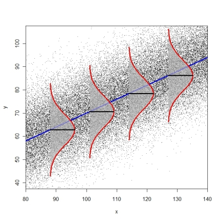
Why is Homoskedasticity Important?
We've talked about $\sigma_\varepsilon$ as the standard deviation of the $\varepsilon_i$ terms. It has an alternate interpretation crucial for the construction of prediction intervals:
-
It is the standard deviation of observations $y$ within a vertical strip, a given point $\tilde{x}$!
-
That is, it gives the estimated standard deviation for $y$ values at a given $\tilde{x}$. $\hat{V}(y^*\mid \tilde{x}) = \hat{\sigma}^2_\varepsilon$.

Why is Homoskedasticity Important?
Homoskedasticity allows us to pool information across residuals (formed at different $x$ values, $x_1,...,x_n$) to calculate an estimate of the standard deviation of $y$ at any point $\tilde{x}$.
If It Was Heteroskedastic...
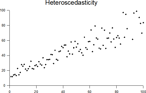
-
In the above scatterplot, if we used $\hat{\sigma}_\varepsilon$ to assess prediction accuracy at $\tilde{x}=10$, would $\hat{\sigma}_\varepsilon$ be larger than or smaller than the actual variability of the vertical strip?
-
What about for $\tilde{x}=40$? For $\tilde{x}=90$?
Plugging in $\hat{\sigma}_\varepsilon$
Consider predicting a future observation $y^*$ at $\tilde{x}$. Consider the random variable
\begin{align*} T = \frac{y^*-\hat{\mu}_{y\mid \tilde{x}}}{\hat{\sigma}_\varepsilon\sqrt{1 + \tilde{x}^\top(X^\top X)^{-1}\tilde{x}}} \end{align*}-
We can compute the center by plugging in $\tilde{x}$ into our estimated prediction equation
-
We can compute the denominator using $\hat{\sigma}_\varepsilon$, $\tilde{x}$, and our design matrix $X$
Under the stronger linear model (when we assume $\varepsilon_i$ are iid and normal), $T$ follows a $t_{n-p-1}$ distribution.
Forming the Prediction Interval
Consider the random variable
\begin{align*} \frac{y^*-\hat{\mu}_{y\mid \tilde{x}}}{\hat{\sigma}_\varepsilon\sqrt{1 + \tilde{x}^\top(X^\top X)^{-1}\tilde{x}}} \end{align*}Because this statistic follows a $t_{n-p-1}$ distribution, it follows that
\begin{align*} (1-\alpha) &= P\left(-t_{1-\alpha/2,n-p-1} \leq \frac{y^*-\hat{\mu}_{y\mid \tilde{x}}}{\hat{\sigma}_\varepsilon\sqrt{1 + \tilde{x}^\top(X^\top X)^{-1}\tilde{x}}} \leq t_{1-\alpha/2,n-p-1}\right) \end{align*}Forming the Prediction Interval
Re-arranging, we find that with probability $(1-\alpha)$, a future observation $y^*$ with covariates $\tilde{x}$ falls within the following interval:
Prediction Intervals
\begin{align*} PI_{100(1-\alpha)\%} &= \hat{\mu}_{y\mid \tilde{x}} \pm t_{1-\alpha/2,n-p-1}\hat{\sigma}_\varepsilon\sqrt{1 + \tilde{x}^\top(X^\top X)^{-1}\tilde{x}} \end{align*}An Example: Opening a New Store
I'm interested in opening a store in a new mall, where there are:
- 3 competitors
- The median income was 75K
Find a 95% prediction interval for this future store. Help me understand the range of sales/sqft I might expect!
xnew = data.frame(income = 75, competitors = 3)
predict(lm.both, newdata = xnew, interval ="prediction",
level = .95)
       fit      lwr      upr
1 578.1509 441.0814 715.2204
First column is the predicted value. Second and third are lower and upper bounds for the prediction interval.
Approximate Prediction Intervals
An approximation to the prediction intervals produced by R (appropriate when
$n$ is large) is given by
Approximation ignores
-
Randomness in $\hat{\sigma}_{\varepsilon}$
-
Randomness in $\hat{\beta}_0 + \hat{\beta}_1\tilde{x}_1+...+\hat{\beta}_p\tilde{x}_p$
Approximate Prediction Intervals
When $n$ is large, $\hat{\sigma}_{\varepsilon}$ closely approximates $\sigma_\varepsilon$, and randomness in the center of interval is small relative to $\sigma_\varepsilon$
-
No reason to use these if you have the data in
R. Use thepredictfunction instead... -
If all you have is the output from
lm, this would be a reasonable approximation.
Empirical Rules for Predictions
We have the following rough/approximate empirical rules, appropriate when $n$ is large. At a given value of $\tilde{x}$, under the stronger linear model,
-
50% of future responses will fall within $\pm \frac{2}{3} \hat{\sigma}_\varepsilon$ from their predicted value, $\hat{\beta}_0 + \hat{\beta}_1\tilde{x}_1 + ... +\hat{\beta}_p\tilde{x}_p$
-
68% of future responses will fall within $\pm 1 \hat{\sigma}_\varepsilon$ from their predicted value, $\hat{\beta}_0 + \hat{\beta}_1\tilde{x}_1 + ... +\hat{\beta}_p\tilde{x}_p$
-
95% of future responses will fall within $\pm 2 \hat{\sigma}_\varepsilon$ from their predicted value, $\hat{\beta}_0 + \hat{\beta}_1\tilde{x}_1 + ... +\hat{\beta}_p\tilde{x}_p$
-
99.7% of future responses will fall within $\pm 3 \hat{\sigma}_\varepsilon$ from their predicted value, $\hat{\beta}_0 + \hat{\beta}_1\tilde{x}_1 + ... +\hat{\beta}_p\tilde{x}_p$
Prediction vs Confidence Intervals
We've recently introduced (1) prediction intervals for future observations $y^*$ at a point $\tilde{x}$; (2) and confidence intervals for $E(y\mid \tilde{x}) = \mu_{y\mid \tilde{x}}$
Prediction Interval for $y^*$
\begin{align*} \hat{\mu}_{y\mid \tilde{x}} \pm t_{1-\alpha/2,n-p-1}\hat{\sigma}_\varepsilon\sqrt{1 + \tilde{x}^\top(X^\top X)^{-1}\tilde{x}} \end{align*}Confidence Interval for $\mu_{y\mid \tilde{x}}$
\begin{align*} \hat{\mu}_{y\mid \tilde{x}} \pm t_{1-\alpha/2,n-p-1}\hat{\sigma}_\varepsilon\sqrt{\tilde{x}^\top(X^\top X)^{-1}\tilde{x}} \end{align*}Same center, but different width. Prediction intervals are wider (often much wider) than confidence intervals.
Prediction vs Confidence Intervals
-
Variance of $\hat{\mu}_{y\mid \tilde{x}}$, ${\sigma}_\varepsilon^2\tilde{x}^\top(X^\top X)^{-1}\tilde{x}$, tends to zero as $n\rightarrow \infty$
-
Variance used for prediction intervals, ${\sigma}_\varepsilon^2(1+\tilde{x}^\top(X^\top X)^{-1}\tilde{x})$, tends to ${\sigma}_\varepsilon^2$ as $n\rightarrow \infty$.
-
Even if I knew $\beta$ (and hence $\mu_{y\mid \tilde{x}}$), I wouldn't be able to perfectly predict future observations.
Prediction vs Confidence Intervals
The two types of intervals address different questions. Here's an example in the context of our father/son data set
Prediction Interval for $y^*$
-
We are told that a father who is 76 inches tall has a son. Find an interval that characterizes the uncertainty in the height of an individual son.
Confidence Interval for $\mu_{y\mid \tilde{x}}$
-
We are interested in the average height for the population of sons whose fathers are 76 inches tall. Find an interval that characterizes our uncertainty in our estimate of the average height of all sons whose fathers are 76 inches tall.