STATS 413: Lecture 7
-
Testing hypotheses for the slope
-
Confidence intervals for $\beta_j$
-
The (overall) $\cF$-test
Hypothesis Testing for the Slope
Consider a linear model $y=X\beta + \varepsilon$ with $p$ predictors, and suppose we wanted to test whether or not the slope on covariate $x_j$, $\beta_j$, was equal to a particular value:
\[ \mathbf{H_o}: \beta_j = \gamma_0 \]The alternatives take the following form:
\begin{align*} \mathbf{H_a}: & \beta_j < \gamma_0 \text{ one-sided, less than}\\ \mathbf{H_a}: & \beta_j> \gamma_0 \text{ one-sided, greater than}\\ \mathbf{H_a}: & \beta_j \neq \gamma_0 \text{ two-sided} \end{align*}By far the most common hypothesis test for slope coefficients is whether $\beta_j = 0$.
Testing $\beta_j$: Interpretation
As we previously discussed, our interpretation of the slope, $\beta_j$ requires ceteris paribus, i.e. "all else equal"
-
For two individuals who vary in $x_j$ by one unit but have the same values for all of the other predictor variables, we expect the difference in $y$ to be $\beta_j$.
-
The value of $\beta_j$, and its interpretation, are dependent upon the context of the model being fit
-
That is, $\beta_j$'s interpretation is tied to the other predictor variables.
As such, hypothesis test for the null $\beta_j = \gamma_0$ can be thought of as:
-
After controlling / adjusting for the effect of all other predictor variables $\{x_\ell\text{ such that } \ell \neq j\}$, let's assess evidence for whether or not the true slope on the $j^{th}$ variable is $\gamma_0$.
A Stronger Linear Model
While the assumptions that $\text{E}(\varepsilon) = 0$; $\text{Var}(\varepsilon) = \sigma^2_\varepsilon I_{n\times n}$ are enough for unbiasedness and to derive a form for the variance for $\widehat{\beta}$, we'll impose additional restrictions on $\varepsilon$ to derive a sampling distribution for $\widehat{\beta}$.
\begin{align*} y &= X\beta + \varepsilon\\ \varepsilon &\sim \text{MVN}(0, \sigma^2_\varepsilon I_{n\times n}), \end{align*}where $\text{MVN}$ represents the multivariate normal distribution
-
Implies that $\varepsilon_i$ $(i=1,...,n)$ are independent and identically (normally) distributed, with expectation zero and variance $\sigma^2_\varepsilon$
The Model in a Picture with $p=1$
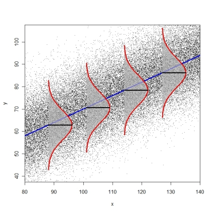
If all three assumptions are met: At any point $x_i$, the population distribution of $y$ values for individuals whose $x$ variable equals $x_i$...
-
Has an expectation of $\beta_0 + \beta_1x_{i1} + ... \beta_p x_{ip} = x_i^\top\beta$ (linearity)
-
Has a standard deviation equal to $\sigma_\varepsilon$ (homoskedasticity)
-
Follows a normal distribution (normality)
The Distribution of $\widehat{\beta}$
Under the stronger linear model (where we assume $\varepsilon_i$ are IID and normally distributed in addition to linearity and homoskedasticity):
\begin{align*} \widehat{\beta}& \sim \text{MVN}(\beta, \sigma^2_\varepsilon (X^\top X)^{-1})\\ \widehat{\beta}_j & \sim N(\beta_j, \sigma^2_\varepsilon (X^\top X)^{-1}_{(j+1),(j+1)}), \end{align*}So for any slope coefficient $j$, letting $\text{SD}(\widehat{\beta}_j) = \sigma_\varepsilon \sqrt{(X^\top X)^{-1}_{(j+1),(j+1)}}$,
\[ \frac{\widehat{\beta}_j-\beta_j}{\text{SD}(\widehat{\beta}_j)} \sim N(0,1) \]Towards a Null Distribution for $\widehat{\beta}_j$
Suppose that the null hypothesis were actually true...
\[ \beta_j = \gamma_0 \]Then, under the null hypothesis and under the stronger linear model,
-
$\text{E}(\widehat{\beta}_j) = \gamma_0$
-
$\text{SD}(\widehat{\beta}_j) = \sigma_{\varepsilon}\sqrt{(X^\top X)^{-1}_{(j+1),(j+1)}}$
Towards the Null Distribution of $\widehat{\beta}_j$
If we knew $\sigma_\varepsilon$:
-
Could begin with the value of the OLS slope coefficient returned by
R, $\widehat{\beta}^{obs}_j$ -
Could define a test statistic $z_{stat} = (\widehat{\beta}^{obs}_j - \gamma_0)/\text{SD}(\widehat{\beta}_j)$
-
Could compute $p$-values using tail probabilities from the normal distribution
Unfortunately, we don't know $\sigma_\varepsilon$ - it is a parameter of the linear model.
-
Can't compute $z_{stat}$, because $\text{SD}(\widehat{\beta}_j)$ depends upon $\sigma_\varepsilon$!
Estimating $\sigma_\varepsilon$
We estimate $\sigma_\varepsilon$ by way of the root mean squared error (RMSE), $\widehat{\sigma}_\varepsilon$
Root Mean Squared Error
\[ \widehat{\sigma}_\varepsilon = \sqrt{\frac{\sum_{i=1}^n e_i^2}{n-p-1}} = \sqrt{\frac{\sum_{i=1}^n (y_i-\widehat{y}_i)^2}{n-p-1}} \]$n-p-1$ are referred to as the degrees of freedom for the residual vector $e$
Estimating $\sigma_\varepsilon$
Why does $e$ have $n-p-1$ degrees of freedom?
-
"How many elements of $e$ are freely determined?"
-
We know that $e$ is constrained by the $p+1$ equations $e^\top X = 0$.
-
Once I tell you $n-p-1$ elements of $e$, the remaining $p+1$ are fixed.
-
Residual vector is constrained to an $n-p-1$ dimensional subspace.
RMSE is referred to as Residual standard error in R output when looking at
summary of an lm object
Standard Errors
We can now estimate $\text{SD}(\widehat{\beta}_j)$ by $\text{se}(\widehat{\beta}_j)$, the standard error for the $j$th coefficient:
\[ \text{se}(\widehat{\beta}_j) = \widehat{\sigma}_\varepsilon \sqrt{(X^\top X)^{-1}_{(j+1), (j+1)}} \]These standard errors are what R gives us when we run summary on an lm
in the second column. We can extract the standard errors as follows:
summary(lm.medicorp)$coefficients[,2]
(Intercept)      Advert       Bonus
179.3557714   0.2563382   0.6904372
A New $t$ Statistic
We'll consider a new test statistic which replaces $\text{SD}(\widehat{\beta}_j)$ with its sample analogue $\text{se}(\widehat{\beta}_j)$
\[ t_{stat} = \frac{\widehat{\beta}_j- \gamma_0}{\text{se}(\widehat{\beta}_j)} \]What's its distribution under the null?
A Null Distribution for Testing $\beta_j$
Under the null hypothesis and assuming the stronger linear model, $t_{stat}$ follows a $t$ distribution with $\mathbf{n-p-1}$ degrees of freedom
A New $t$ Statistic
We then use tail probabilities from the $t_{n-p-1}$ distribution to compute $p$-values. We can get these in
R using the command pt(tstat, n-p-1), which calculates the left tail probability.
Reminder: The $t$ Distribution
The $t$ family of distributions is indexed by a number known as its "degrees of freedom," or $df$ for short. We'll denote a $t$ distribution with $df$ degrees of freedom as $t_{df}$.
-
For different values of the degrees of freedom, we have different $t$ distributions. Different thickness of tails, different quantiles.
-
The smaller the "degrees of freedom", the fatter the tails of the $t$-distribution
-
As $df\rightarrow \infty$, the $t_{df}$ converges to a standard normal distribution.
-
Departure from normality comes from the variability in the denominator of $t_{stat}$ (estimating standard deviation by a standard error)
Reminder: Normal vs $t$ Distribution

The red curve is a normal distribution. The other black curves are actually various $t$ distributions.
Back to the Output
Coefficients:
            Estimate Std. Error t value Pr(>|t|)
(Intercept) -682.3699   179.3558  -3.805 0.000913 ***
Advert         2.6949     0.2563  10.513 2.95e-10 ***
Bonus          2.0970     0.6904   3.037 0.005855 **
---
Signif. codes:  0 '***' 0.001 '**' 0.01 '*' 0.05 '.' 0.1 ' ' 1

Residual standard error: 87.55 on 23 degrees of freedom-
Third column contains test statistics corresponding to the null hypothesis that $\beta_j=0$ (divide first column by second column)
-
Fourth column contains $p$-values for testing $\beta_j=0$ when there's a two-sided alternative.
Back to the Output
summary(lm.medicorp)

Coefficients:
            Estimate Std. Error t value Pr(>|t|)
(Intercept) -682.3699   179.3558  -3.805 0.000913 ***
Advert         2.6949     0.2563  10.513 2.95e-10 ***
Bonus          2.0970     0.6904   3.037 0.005855 **
---
Signif. codes:  0 '***' 0.001 '**' 0.01 '*' 0.05 '.' 0.1 ' ' 1

Residual standard error: 87.55 on 23 degrees of freedom
Example: if we tested the null hypothesis that $\beta_{bonus} = 0$ with a two-sided alternative at $\alpha=0.05$, we'd reject the null and suggest that even after adjusting for advertising spend, locations with higher bonus spends have higher sales.
Another Interpretation of $H_0: \beta_j = 0$
Once again, the null hypothesis $\beta_j = 0$ will be, by far, the most common in practice. There's an alternative interpretation of the test for $\beta_j = 0$:
After controlling for the other predictor variables besides $x_j$, $\{x_\ell : \ell \neq j\}$, is there evidence that $x_j$ substantially improves the predictive power of our model?
-
In other words, do we need to include $x_j$ once we've already included the other $p-1$ variables?
-
If the null, $\beta_j = 0$, is true, the answer is no!
-
All else equal, we often prefer parsimonious models for the sake of interpretation! The simpler the better, unless its worth making the model more complicated
In Our Example...
In our example, both slopes were statistically significantly different from zero at $\alpha = 0.05$
Reject the null that $\beta_{advert} = 0$:
-
There's evidence that
advertprovides a significant improvement in predictive power relative to a model that only includesbonus
Reject the null that $\beta_{bonus} = 0$:
-
There's evidence that
bonusprovides a significant improvement in predictive power relative to a model that only includesadvert
Recap: Distribution for $\widehat{\beta}$
Assume:
\begin{align*} y &= X\beta + \varepsilon\\ \varepsilon_i &\overset{iid}{\sim} N(0, \sigma^2_\varepsilon), \end{align*}We know that $\textbf{E}(\widehat{\beta}) = \beta$, and $\text{Var}(\widehat{\beta}) = \sigma^2_\varepsilon(X^\top X)^{-1}$
-
How would I extract $\text{SD}(\widehat{\beta}_j)$ using $\text{Var}(\widehat{\beta})$?
-
What was the distribution of $\displaystyle\frac{\widehat{\beta}_j - \beta_j}{\text{SD}(\widehat{\beta}_j)}$?
-
What was $\widehat{\sigma}^2_\varepsilon$?
Recap: Distribution for $\widehat{\beta}$
Assume:
\begin{align*} y &= X\beta + \varepsilon\\ \varepsilon_i &\overset{iid}{\sim} N(0, \sigma^2_\varepsilon), \end{align*}We know that $\textbf{E}(\widehat{\beta}) = \beta$, and $\text{Var}(\widehat{\beta}) = \sigma^2_\varepsilon(X^\top X)^{-1}$
-
What was $\text{se}(\widehat{\beta}_j)$?
-
What was the distribution of $\displaystyle\frac{\widehat{\beta}_j - \beta_j}{\text{se}(\widehat{\beta}_j)}$?
$P$-value Computations
Let $t_{stat}$ be my observed test statistic, $t_{stat} = (\widehat{\beta}_j^{obs} - \gamma_0)/\text{se}(\widehat{\beta}_j)$, and let $T_{n-p-1}$ be a random variable which follows a $t_{n-p-1}$ distribution. To calculate $p$-values:
-
Less than alternative: $p_{val} = P(T_{n-p-1} \leq t_{stat})$
-
Greater than alternative: $p_{val} = P(T_{n-p-1} \geq t_{stat}) = 1 - P(T_{n-p-1} \leq t_{stat})$
-
Two-sided alternative: \begin{align*} p_{val} &= P(|T_{n-p-1}| \geq |t_{stat}|)\\ &= P(T_{n-p-1} \geq |t_{stat}|) + P(T_{n-p-1} \leq -|t_{stat}|)\\ &= 2P(T_{n-p-1} \geq |t_{stat}|) = 2P(T_{n-p-1} \leq -|t_{stat}|) \end{align*} (Last two identities use the fact that the $t$ distribution is symmetric)
Quantifying Uncertainty
Let $t_{1-\alpha/2, n-p-1}$ represent the $(1-\alpha/2)$ quantile from a $t$ distribution with $n-p-1$ degrees of freedom.
-
By symmetry of $t$ distribution: $-t_{1-\alpha/2,n-p-1} = t_{\alpha/2, n-p-1}$
Under our stronger linear model (linearity, homoskedasticity, normality), we have that
\[ \frac{\widehat{\beta}_j-\beta_j}{\text{se}(\widehat{\beta}_j)} \sim t_{n-p-1} \]Quantifying Uncertainty
Implies for $\alpha \leq 0.5$:
\begin{align*} 1-\alpha &= P\left(-t_{1-\alpha/2, n-p-1} \leq \frac{\widehat{\beta}_j-\beta_j}{\text{se}(\widehat{\beta}_j)} \leq t_{1-\alpha/2, n-p-1}\right) \\ & = P\left(\widehat{\beta}_j - t_{1-\alpha/2, n-p-1}\text{se}(\widehat{\beta}_j) \leq \beta_j \leq \widehat{\beta}_j + t_{1-\alpha/2, n-p-1}\text{se}(\widehat{\beta}_j)\right) \end{align*}Confidence Intervals for $\beta_j$
Provided the assumptions for the (stronger) linear model hold (linearity, homoskedasticity, normality of $\varepsilon$):
Confidence Intervals for $\beta_j$
A $100(1-\alpha)\%$ $t$-based confidence interval for $\beta_j$ is:
\[ \widehat{\beta}_j \pm t_{1-\alpha/2, n-p-1}\text{se}(\widehat{\beta}_j) \]Confidence Intervals for $\beta_j$
We find $t_{1-\alpha/2, n-p-1}$ through running qt(1-alpha/2, n-p-1) in R.
Example: a 95% confidence interval for the slope on bonus is:
> 2.10 + c(-1,1)*qt(.975, n-2-1)*0.69
  [1] 0.6726262 3.5273738
Confidence Intervals in R
R makes it easy to compute confidence intervals for slope coefficients at any confidence level:
> confint(lm.medicorp, level = .95)
                  2.5 %      97.5 %
(Intercept) -1053.3956070 -311.344244
Advert          2.1646581    3.225210
Bonus           0.6687373    3.525294
Interpreting a Confidence Interval
We now have the machinery required to create a 95% (or any %) confidence interval
-
Suppose we have a data set, and the mean of our variable was $\widehat{\beta}_j^{obs}$.
-
Our 95% confidence interval would simply be $\widehat{\beta}_j^{obs} \pm t_{0.975, n-p-1} \text{se}(\widehat{\beta}_j)$.
-
How do we express this result in English?
Interpreting a Confidence Interval
Expressing Confidence Intervals
If our confidence interval is $\widehat{\beta}_j^{obs} \pm t_{0.975, n-p-1} \text{se}(\widehat{\beta}_j)$, we say that "we are 95% confident that $\beta_j$, the true population slope, falls between $\widehat{\beta}_j^{obs} - t_{0.975, n-p-1} \text{se}(\widehat{\beta}_j)$ and $\widehat{\beta}_j^{obs} + t_{0.975, n-p-1}\text{se}(\widehat{\beta}_j)$"
Values for $\beta_j$ which are outside the interval appear unlikely/implausible.
What Does Confidence Mean? What's Random?
If I observe $\widehat{\beta}_j = \widehat{\beta}_j^{obs}$, we say that we are 95% confident that $\beta_j$ falls within an interval of the form $\widehat{\beta}_j^{obs} \pm t_{0.975, n-p-1} \text{se}(\widehat{\beta}_j)$...
-
Is $\beta_j$ random?
-
Is $\widehat{\beta}_j$ random?
-
Is $\text{se}(\widehat{\beta}_j)$ random?
-
So what's random here? THE INTERVAL!
How is the interval random? Across data sets / draws from the linear model.
What Does Confidence Mean? What's Random?
-
For each data set, we see one random sample slope, $\widehat{\beta}_j$, and a random standard error estimator $\text{se}(\widehat{\beta}_j)$
-
If I had collected another data set, I would have had a different vector $\widehat{\beta}$ and a different standard error $\text{se}(\widehat{\beta}_j)$, because I would have had different respondents in my sample
-
Hence, my interval $\widehat{\beta}_j \pm t_{0.975, n-p-1} \text{se}(\widehat{\beta}_j)$ is random, because it varies from data set to data set!
-
Our data set is one "possible world." We usually only collect one data set, but the data set could have been different, and that's the point!
-
Across 95% of data sets, a 95% confidence interval will capture the true value of $\beta_j$.
Visualizing the Probabilistic Interpretation
Imagine trying to estimate and construct confidence intervals for the true slope coefficient, $\beta_j = 2.1$, using multiple regression:

Another Valid Interpretation
A Probabilistic Interpretation of a 95% Confidence Interval
Suppose I'm a data analyst, and each day I'm given a new data set. This data set need not arise from the same distribution from one day to the next (you could be given data from different populations, and asked to conduct different regressions)
-
For each data set, I construct a 95% confidence interval for the value of a slope coefficient, $\beta_j$
95% of days, my confidence interval will have successfully captured the true slope
Connecting CIs and Hypothesis Tests
We've talked about Confidence Intervals and Hypothesis Tests.
-
Argued that if a value $\gamma_0$ fell outside of the $100(1-\alpha)\%$ confidence interval for $\beta_j$ based on our sample, then it seems unlikely that $\gamma_0$ was possibly the true slope
-
For hypothesis testing, we postulate a value for $\gamma_0$, and decide to reject or fail to reject it based on whether our $p$-value is less than or equal to $\alpha$, our significance level.
Connecting CIs and Hypothesis Tests
These sure do seem to be answering very similar questions. Is there a connection?
-
Turns out that if our alternative is two-sided and we conduct a test with significance level $\alpha$, we can reject the null $\gamma_0$ if and only if $\gamma_0$ does not fall within the $100(1-\alpha)\%$ confidence interval.
-
Correspondingly, $\gamma_0$ is in our confidence interval if and only if we failed to reject the null that $\beta_j = \gamma_0$ with a two sided alternative
Making it Formal
For a two-sided alternative, we fail to reject the null hypothesis $\beta_j = \gamma_0$ if and only if our test statistic does not exceed $t_{1-\alpha/2, n-p-1}$ in absolute value.
We fail to reject if and only if $|t_{stat}| \leq t_{1-\alpha/2, n-p-1}$:
\begin{align*} -t_{1-\alpha/2, n-p-1} &\leq t_{stat} \leq t_{1-\alpha/2, n-p-1}\\ -t_{1-\alpha/2, n-p-1} &\leq \frac{\widehat{\beta}_j - \gamma_0}{\text{se}(\widehat{\beta}_j)} \leq t_{1-\alpha/2, n-p-1}\\ -t_{1-\alpha/2, n-p-1}\text{se}(\widehat{\beta}_j) & \leq \widehat{\beta}_j - \gamma_0 \leq t_{1-\alpha/2, n-p-1}\text{se}(\widehat{\beta}_j)\\ \widehat{\beta}_j - t_{1-\alpha/2, n-p-1}\text{se}(\widehat{\beta}_j) & \leq \gamma_0 \leq \widehat{\beta}_j + t_{1-\alpha/2, n-p-1}\text{se}(\widehat{\beta}_j) \end{align*}Making it Formal
For a two-sided alternative, we fail to reject the null hypothesis $\beta_j = \gamma_0$ if and only if our test statistic does not exceed $t_{1-\alpha/2, n-p-1}$ in absolute value.
We fail to reject if and only if $|t_{stat}| \leq t_{1-\alpha/2, n-p-1}$:
\begin{align*} \widehat{\beta}_j - t_{1-\alpha/2, n-p-1}\text{se}(\widehat{\beta}_j) & \leq \gamma_0 \leq \widehat{\beta}_j + t_{1-\alpha/2, n-p-1}\text{se}(\widehat{\beta}_j) \end{align*}This last line says that we fail to reject if and only $\gamma_0$ is in $\widehat{\beta}_j \pm t_{1-\alpha/2, n-p-1}\text{se}(\widehat{\beta}_j)$. This is the definition of a $100(1-\alpha)\%$ confidence interval!
Implication and Example
Implication: If we have, say, a 95% confidence interval, we can check whether or not we'd reject any value of $\beta_j=\gamma_0$ with a two sided alternative at significance level 0.05 just by looking at the 95% confidence interval!
-
An example: Suppose I found that my 95% confidence interval for $\beta_j$ was $[1, 7]$.
-
Then, at significance level $\alpha = 0.05$ I know that I would fail to reject the null hypothesis that $\beta_j = 5$ vs the alternative that $\beta_j \neq 5$ since it falls within the confidence interval
-
And, at significance level $\alpha = 0.05$ I know that I would reject the null that $\beta_j = 10$ vs the alternative that $\beta_j \neq 10$ since it doesn't fall within the confidence interval