STATS 413: Lecture 6
-
Quantifying model fit: SSE, SST, and $R^2$
-
Testing statistical hypotheses
-
Testing hypotheses for the slope
Quantifying Errors
We'll now introduce a few summary measures related to variability in the residuals in order to:
-
Characterize how much variability in our outcomes cannot be accounted for by our predictor variables
-
Asses quality of model fit.
-
Come up with an estimator for $\sigma^2_\varepsilon$, a necessary step when (a) performing inference; and (b) constructing prediction intervals for future observations.
The Sum of Squared Errors
Define the sum of squared errors (SSE) as follows:
Sum of Squared Errors (SSE)
\begin{align*} \text{SSE} &=\textstyle \sum_{i=1}^n e_i^2 = \sum_{i=1}^n(y_i-\hat{y}_i)^2\\ &= {e}^\top e = {(y-X\hat{\beta})}^\top (y-X\hat{\beta}) \end{align*}(important to become comfortable with equivalent representations of quantities, and to understand why they are equivalent)
The Sum of Squared Errors
This value is equal to
\begin{align*}\min_{\beta}{(y-X\beta)}^\top (y-X\beta), \end{align*}since the OLS coefficients $\hat{\beta}$ are the values of $\beta$ that minimize this expression
The Total Sum of Squares (SST)
The total sum of squares represents the total variability in $y$ itself, without trying to predict using our explanatory variables
Total Sum of Squares (SST)
\begin{align*} \text{SST} &=\textstyle \sum_{i=1}^n (y_i - \bar{y})^2\\ &= (n-1)\text{var}(y) = (n-1)\text{sd}(y)^2, \end{align*}where $\text{var}(y)$ is the sample variance of $y$ and $\text{sd}(y)$ the sample standard deviation of $y$.
Aside: Regression with Only an Intercept
Suppose I didn't have any predictor variables, but that I nonetheless wanted to run a regression.
\begin{align*} y_i &= \beta_0 + \varepsilon_i \end{align*}For this regression...
-
The design matrix $X$ is simply a vector containing $n$ ones (only the intercept column).
-
The estimated intercept $\hat{\beta}_0$ would be $\bar{y}$
-
$\hat{y}_i = \bar{y}$ for all individuals
-
The residuals from this regression would be $e_i = y_i-\bar{y}$
Interpreting SST
From the view of a regression with only an intercept:
Total Sum of Squares (SST)
\[\textstyle \text{SST} = \sum_{i=1}^n (y_i - \bar{y})^2 \]The $\text{SST}$ is the sum of squared errors in a regression that doesn't include any of the predictor variables, and instead only uses an intercept.
Interpreting SSE
Recall that $\text{SSE}$ is the sum of squared errors in a regression that does use the predictor variables.
-
Answers the question: how much error in $y$ is left over after forming predictions using our explanatory variables $X$?
What would a comparison of $\text{SSE}$ to $\text{SST}$ inform us of?
$R^2$ (Coefficient of Determination)
We form a numerical quantity called $R^2$, which helps measure the predictive power of our linear model
$R^2$
\[ R^2 = 1 - \frac{\text{SSE}}{\text{SST}} \]The $R^2$ value is the fraction of variation in the outcome variable $y$ that can be accounted for by our predictor variables $X$ through our linear model
$R^2$ (Coefficient of Determination)
It quantifies how much "better" we are doing in prediction by using our linear model than we would have been stuck with in the absence of any predictor variables (predict the overall mean for all individuals)
Properties of $R^2$
-
$0 \leq R^2 \leq 1$
-
Consequence of $\text{SSE}\leq \text{SST}$. Do you see why this holds?
-
-
$R^2 = \text{cor}(\hat{y}, y)^2$
-
In simple regression $(p=1)$, simplifies to $R^2 = \text{cor}(x, y)^2$.
-
-
$R^2$ never decreases as you add more predictor variables in to your regression (even if the predictors are irrelevant!).
Measures the strength of the linear relationship between responses and predictors. Not an appropriate summary measure under model misspecification.
Remarks on $R^2$
$R^2$ near $0$ could be either of the following:

Remarks on $R^2$
$R^2$ small does not mean that $y$ and $X$ are not linearly related (can have slight trend with lots of leftover variability).

$R^2$ is equal to 0.2.
Remarks on $R^2$
Likewise, $R^2$ close to $1$ does not mean the linear model is correct.

$R^2$ is equal to 0.9.
Anscombe's Quartet
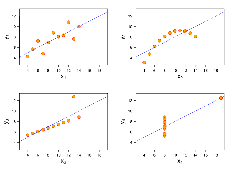
All have the same $R^2$ of 0.67! VISUALIZE YOUR DATA
Medicorp
Medicorp Company sells medical supplies. The company markets in three regions of the United States. Medicorp's management is concerned with the effectiveness of a new bonus program and the effectiveness of the advertisement. The bonus is provided to sales representatives based on the performance. Management conducts a study to answer the following questions:
-
Do the average sales for their national locations exceed 1.2 million?
-
After adjusting for differences in advertising spend, is there evidence that locations which differ in their bonus payments differ in sales?
-
After adjusting for differences in bonus spend, is there evidence that locations which differ in advertising spend differ in average sales?
Medicorp
The variables considered in this study include:
-
Sales: Medicorp's sales (in thousands of dollars) from each location for 1999. -
Advert: The amount spent on advertising in each location (in hundreds) in 1999. -
Bonus: The total amount paid in bonus in each location (in hundreds) in 1999. -
Region: South, West and Midwest.
The data comes from a simple random sample of 26 locations.
Recap: Hypothesis Testing
When conducting statistical inference, we are informally trying to answer the following question:
-
Is what I'm observing real, or could it be attributable to random chance alone?
Our pursuit begins with both a question which we collect data to try to answer
-
The Alternative Hypothesis is what we, the researcher, want to show
-
The Null Hypothesis is the opposite of what we want to show. Oftentimes, this represents the status quo. The purpose of research is often to further knowledge by refuting this commonly held belief
The Scientific Method
Knowledge is acquired by the postulation of testable hypotheses, which aim to modify the current state of knowledge
-
In order to prove a new hypothesis, one does not actually collect evidence to confirm it
-
Rather, we proceed backwards: data is collected to falsify the opposite of what we want to prove
-
We end up using a device known as a proof by contradiction
-
Technique is known as empirical refutation/falsification, espoused by Karl Popper.
American Criminal Justice
Suppose a murder has been committed and the defendant is accused.
-
The prosecutor (researcher) wants to prove the hypothesis that the defendant is guilty (i.e., to show that innocence is implausible)
-
The prosecutor collects evidence to falsify the opposite of what he believes (innocence, the value under the null).
-
The assumption is that the defendant (the null hypothesis) is innocent until proven guilty. The burden of proof is on the prosecutor (researcher) to show that the hypothesis of innocence is untenable given the evidence (data)
American Criminal Justice
How is a decision made?
-
All of the evidence (data) is evaluated. If the null hypothesis of innocence is completely untenable given the evidence (data), it is rejected in favor of the alternative hypothesis of guilt
-
If the evidence (data) does not show implausibility of innocence (the null) beyond a reasonable doubt, we fail to reject the null hypothesis of innocence.
-
It's not to say that innocence (the null) is the reality. Rather, we simply lack enough evidence to refute it. The verdict is "not guilty" rather than "innocent"
-
An important distinction!
Tests of Significance
The statistician gets to play the role of judge in assessing whether random chance alone could yield the observed evidence
The statistician has invented tests to help decide if the data is so inconsistent with the null hypothesis that it should be declared false
Tests of Significance
This involves a statistical hypothesis test:
-
If the null hypothesis were true, what's the chance of observing evidence as extreme or more extreme than what we observed in our data if randomness alone were the explanation?
-
If this probability, the p-value, is too small (i.e., the discrepancy is so large), then it seems like randomness/chance variation alone is an unreasonable explanation.
-
In that case, we would say that a more likely cause is that the null hypothesis doesn't appear to be true! We would reject the null hypothesis, and suggest that our alternative hypothesis provides a more reasonable explanation
Proof by Contradiction
We will go about trying to disproving the null hypothesis through the following process..
-
Begin by assuming that the null is true
-
Under the assumption that the null is true, we evaluate how likely it is to observe a result that is as extreme or more extreme than the one we observed in our data
-
If we determine that this probability is "significantly small," we will then suggest that since the data would be improbable under the null, the assertion that the null is true seems implausible
Reminder: Test Statistics and $p$-values
Hypothesis tests involve the formation of a test statistic
-
Quantity that relates to the degree of "evidence" against the null hypothesis
How do we make a decision? We ask ourselves the following question:
-
How unlikely would it be to observe a test statistic like the one I saw in my data if the null was true?
-
Could a deviation of this type be explained by chance randomness alone? We answer this question with a probability, known as a $p$-value:
Reminder: Test Statistics and $p$-values
$p$-value (in words)
A $p$-value is defined to be the probability of observing a result that is as extreme or more extreme than what we have actually observed in our sample or experiment, given that the null hypothesis is actually true.
What the $p$-value is NOT
The $p$-value is NOT the probability that null hypothesis is true.
-
It is the probability of finding a result as extreme or more extreme that what we observed in our sample if the null hypothesis were true.
These are very different things.
-
The probability that the null is true is either 0 or 1.
-
It either is or it isn't, in the same way that the population mean is either in your confidence interval or it isn't.
-
The truth of the null hypothesis is constant. It either is or it isn't, we just don't know which of these potential truths is the true truth.
Significance Level
Once we compute the appropriate $p$-value, we need to determine if it is substantial enough to reject the null hypothesis
-
We will reject if the $p$-value is substantially small
Significance Level
But what is substantial? We define a $p$-value to be "significant" if it falls at or below a pre-specified significance level
Significance Level
The significance level of a hypothesis test, denoted as $\alpha$, is a significance threshold specified before the analysis begins such that if the $p$-value falls at or below $\alpha$, we reject the null hypothesis
-
Convention is to use $\alpha = 0.05$.
Making a Decision
If $p$-value that we calculate is less than or equal to $\alpha$, then we deem that the observed evidence was statistically significantly different from what we would have expected to see under the null. We reject the null hypothesis.
-
That is, we suggest that the deviation of what we observed from what would be typical under the null is too large to be explained by randomness alone.
-
Hence, if we observe a $p$-value that is less than or equal to $\alpha$, we have sufficient evidence to reject the null and suggest that the alternative hypothesis appears to be more plausible.
Making a Decision
If our $p$-value is greater than $\alpha$, then we say we fail to reject the null hypothesis.
-
We lack sufficient evidence to reject the null hypothesis
-
The result observed could still reasonably be attributed to random chance alone under the null
Can Never Accept the Null
Note that our options are either:
-
Reject the null
-
Fail to reject the null
We can never say that we "accept" the null if our $p$-value is greater than $\alpha$.
-
If our proof by contradiction fails, it doesn't mean we've proven the thing we were trying to contradict. Rather, we simply lack enough evidence to disprove it.
-
In the same way, just because someone was acquitted doesn't mean we really think they are innocent; rather, we didn't have strong enough evidence to prove their guilt.
Imperfect Decision Making
We decide to reject or fail to reject a null hypothesis based on whether or not $p\text{-value} \leq \alpha$.
-
The $p$-value is the probability of observing something as extreme or more extreme than what we observed in our sample if the null hypothesis is true...
Imperfect Decision Making
Doesn't that mean there's still a chance that the null is true, even if we decide to reject it?
-
Yes! We can never know for certain whether the null is true.
By the same token, if we fail to reject the null, is it still possible that the null is false?
-
Yes! Failure to reject the null simply means we lacked sufficient evidence to reject it. It doesn't speak to its validity or invalidity
Types of Errors
We can characterize the types of correct or incorrect decisions in a $2\times 2$ table:
| Fail to Reject the Null | Reject the Null | |
|---|---|---|
| $\mathbf{H_0}$ is actually true | No error | Type I error |
| $\mathbf{H_0}$ is actually false | Type II error | No error |
A Type I Error occurs if we reject the null hypothesis when it was actually true
-
In our courtroom "innocent until proven guilty" example, this would be declaring the defendant guilty, when he was actually innocent
Types of Errors
We can characterize the types of correct or incorrect decisions in a $2\times 2$ table:
| Fail to Reject the Null | Reject the Null | |
|---|---|---|
| $\mathbf{H_0}$ is actually true | No error | Type I error |
| $\mathbf{H_0}$ is actually false | Type II error | No error |
A Type II Error occurs if we fail to reject the null hypothesis when it was actually false
-
This would be declaring the defendant not guilty, when he was actually guilty
Type I and Type II Errors
The significance level directly determines the Type I error rate.
-
We reject the null hypothesis when $p\text{-value} \leq \alpha$.
-
If the null is true, $P(\text{Type I Error}) \leq \alpha$
Type II errors are a practitioner's nightmare. Their suspicion that the null was incorrect is actually true, but they weren't able to show it based on their test!
-
The null was incorrect, but they failed to reject it
-
For a given significance level, increasing sample size $n$ increases the power of a well-designed test
Generally, we try to devise tests that have the largest power possible, subject to controlling the Type I Error rate at $\alpha$.
Recap: One-Sample Hypothesis Testing for the Mean
The management at Medicorp wants to see if average sales at their locations exceed $1.2 Million.
-
What's the null hypothesis?
-
What's the alternative?
-
What test statistic would we consider using if we knew the true standard deviation of sales?
Recap: One-Sample Hypothesis Testing for the Mean
The management at Medicorp wants to see if average sales at their locations exceed $1.2 Million.
-
What would its distribution be (at least approximately) under the null hypothesis?
-
What test statistic do we use instead, recognizing that the true standard deviation is typically unknown?
-
What was its distribution under the null hypothesis?
-
How do we compute a $p$-value?
Recap: One-Sample Hypothesis Testing for the Mean
The management at Medicorp wants to see if average sales at their locations exceed $1.2 Million.
-
What's the null hypothesis?
-
What's the alternative?
-
What test statistic would we consider using if we knew the true standard deviation of sales?
-
What would its distribution be (at least approximately) under the null hypothesis?
-
What test statistic do we use instead, recognizing that the true standard deviation is typically unknown?
-
What was its distribution under the null hypothesis?
-
How do we compute a $p$-value?
New Hypothesis Tests
Medicorp further wants to understand the impact of advertising spend and bonus spend on sales.
-
After adjusting for differences in advertising spend, is there evidence that locations which differ in their bonus payments differ in sales?
-
After adjusting for differences in bonus spend, is there evidence that locations which differ in advertising spend differ in average sales?
They imagine the following linear model holds for the conditional expectation of sales:
\[ \text{E}(\texttt{Sales}\mid \texttt{Advert}, \texttt{Bonus}) = \beta_0 + \beta_{\texttt{advert}}\texttt{Advert} + \beta_{\texttt{bonus}}\texttt{Bonus} \]Can we relate the company's questions to parameters in the above model?
Output from R
summary(lm.medicorp)

Coefficients:
            Estimate Std. Error t value Pr(>|t|)
(Intercept) -682.3699   179.3558  -3.805 0.000913 ***
Advert         2.6949     0.2563  10.513 2.95e-10 ***
Bonus          2.0970     0.6904   3.037 0.005855 **
---
Signif. codes:  0 '***' 0.001 '**' 0.01 '*' 0.05 '.' 0.1 ' ' 1

Residual standard error: 87.55 on 23 degrees of freedom
We already understand the first column here (contains $\widehat{\beta}$). The remainder are useful for performing hypothesis tests...