STATS 413: Lecture 3
-
Estimation for linear models
-
Interpreting Regression Parameters
The Multiple Regression Problem
In general, our responses $y_i$ might be thought of as functions of $p>1$ explanatory variables
We'd like to fit a function of the form:
\[ \hat{y}_i = \hat{\beta}_0 + \hat{\beta}_1x_{i1} + \hat{\beta}_2x_{i2}+ \dots +\hat{\beta}_px_{ip} \]How should we choose these coefficients?
-
In simple regression $(p=1)$, we chose the values $\hat{\beta}_0$ and $\hat{\beta}_1$ that minimized the sum of squared residuals:
\[\textstyle (\hat{\beta_0}, \hat{\beta}_1) = \arg\min_{\beta_{0}, \beta_{1}}\;\; \sum_{i=1}^n(y_i - (\beta_0 + \beta_1x_i))^2 \]
Let's extend this criterion to multiple dimensions
Finding the Least Squares Regression Line
We again consider distances between observed values, $y_i$, and predicted values, ${\beta}_0 + {\beta}_1x_{i1}+...+{\beta}_px_{ip}$ for different choices of $\beta = (\beta_0,\beta_1,...,\beta_p)$
Solution through Optimization
The least squares coefficients $\hat{\beta}_0, \hat{\beta}_1,\dots,\hat{\beta}_p$ are
\[\textstyle \underset{\beta_0, \beta_1,...,\beta_p}{\arg \min}\;\;\sum_{i=1}^n(y_i - (\beta_0 + \beta_1x_{i1} + ... + \beta_{p}x_{ip}))^2 \]Finding the Least Squares Regression Line
R produces the solution using the lm command.
lm(y~x1+x2+...+xp)
Python offers multiple approaches. Using scikit-learn:
from sklearn.linear_model import LinearRegression
model = LinearRegression()
model.fit(X, y)  # X is n×p matrix of predictors
or using statsmodels for statistical output similar to R:
import statsmodels.api as sm
X_with_const = sm.add_constant(X)  # adds intercept
model = sm.OLS(y, X_with_const).fit()
Multiple Regression in Our Example
lm(sales~competitors+income)

Coefficients:
(Intercept)  competitors       income
     91.422      -25.135        7.495
Example: For a mall with two competitor stores and and a surrounding area with a median income of 57 thousand dollars, we'd predict the sales per square foot to be
\[ \widehat{\mathtt{sales}} = 91.42 - 25.14\times 2 + 7.50\times 57 = 468.6 \]Additional Quantities
-
Fitted values for the $n$ observations in our data set
\[ \hat{y}_i = \hat{\beta}_0 + \hat{\beta}_1 x_{i1} + \dots + \hat{\beta}_p x_{ip}\;\; (i=1,\dots,n) \] -
Fitted model (for forming predictions at other values of ${x}$ beyond those in our data).
\[ \hat{f}({x}^*) = \hat {\beta}_0 + \hat{\beta}_1 x^*_{1} + \dots + \hat{\beta}_p x^*_{p} \\ \] -
Residuals:
\[ e_i = y_i - \hat{y}_i \;\; (i=1,\dots,n) \]
Additional Quantities
Note that
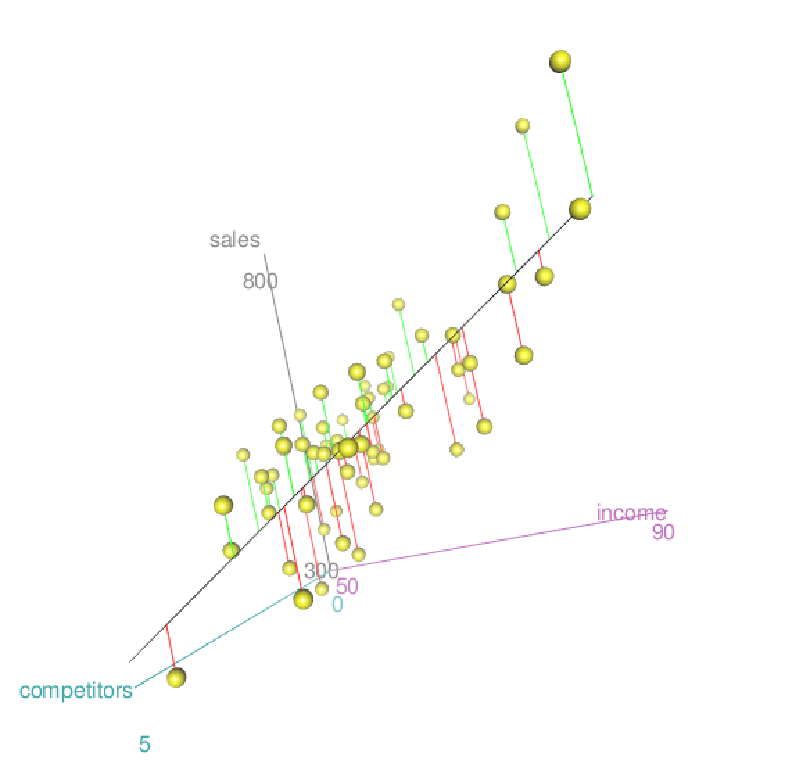
\[\textstyle \sum_{i=1}^n e_i^2 = \underset{\beta_0, \beta_1,...,\beta_p}{\min}\;\;\sum_{i=1}^n(y_i - (\beta_0 + \beta_1x_{i1} + ... + \beta_{p}x_{ip}))^2 \]Estimated Response Surface and the Residuals
Here's a visualization of a multiple regression with sales as the response and
compet and income as the two predictor variables.
Plane of Best Fit
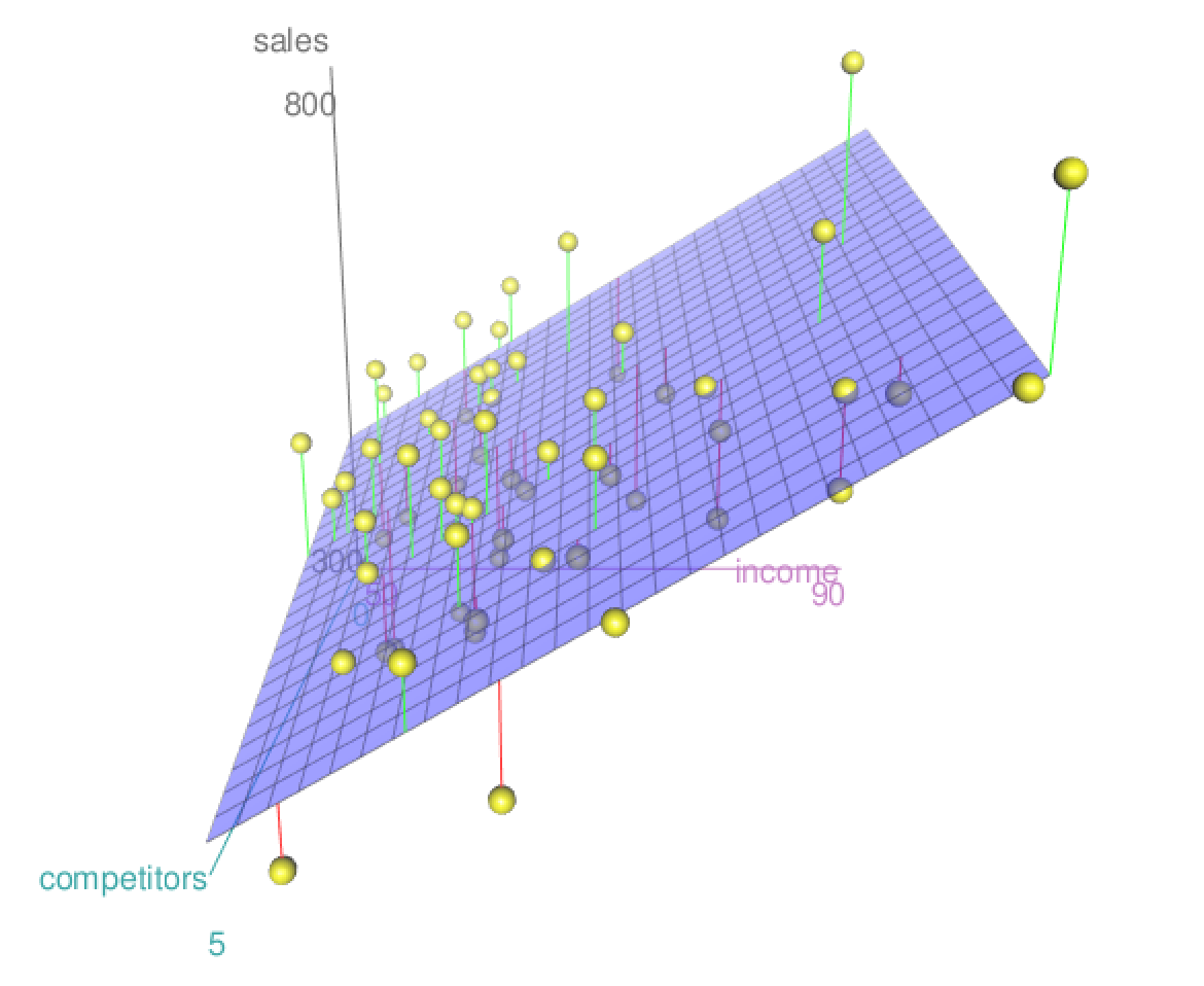
Residuals (sales - predicted sales)
More Advanced Output
summary(lm.both)

Coefficients:
            Estimate Std. Error t value Pr(>|t|)
(Intercept)  91.4221    53.2652   1.716 0.091172 .
competitors -25.1345     6.3667  -3.948 0.000207 ***
income        7.4951     0.8909   8.413  8.6e-12 ***
---
Signif. codes:  0 '***' 0.001 '**' 0.01 '*' 0.05 '.' 0.1 ' ' 1

Residual standard error: 67.42 on 61 degrees of freedom
Multiple R-squared:  0.5384,	Adjusted R-squared:  0.5233
F-statistic: 35.58 on 2 and 61 DF,  p-value: 5.748e-11
What does all this mean? We'll need to develop some theory to understand this output...
General Objective in Regression
We begin by postulating a generative model, which describes how our observed data $({x}_1, y_1), \dots, ({x}_n, y_n)$ came to be.
-
Relate the observed data to parameters of our population of interest.
-
Through using the data, we try to infer the values of the parameters for the population of interest.
General Objective in Regression
General form for this generative model states that, for $i=1,\dots,n$,
\[ y_i = f(x_i) + \varepsilon_i;\;\; (i=1\dots,n) \]where
-
$f(x_i) \triangleq \textbf{E}(y_i \mid x_i)$ is the (unknown) regression function (ie the signal) relating expected response to predictors
-
$\varepsilon_i$ are random noise terms such that $\textbf{E}(\varepsilon_i\mid x_i)=0$.
Objectives
-
estimate $f$ using observed data, resulting in estimated function $\hat{f}$
-
estimate the conditional distribution $Y_i\mid {x}_i$
Linear Regression Analysis
-
We generally impose some restrictions/structure on $f(\cdot)$.
-
For linear models, we assume \[ f(x_i) = \textbf{E}(y_i\mid {x}_i) = \beta_0 + \beta_1 x_{i,1} + \cdots + \beta_p x_{i,p}, \] where $\beta_1,\dots,\beta_p$'s are (unknown) regression coefficients and $\beta_0$ is the (also unknown) intercept.
-
estimation of $f(\cdot)$ is equivalent to estimation of $\beta_j$'s
Transformation
Linear models are much less restrictive than you might think.
-
They can be made very flexible by transformation of the response and the predictors.
Example (account for curvature): suppose I wanted to use linear regression to fit the equation
\[ \hat{f}(x) = \hat{\beta}_0 + \hat{\beta}_1x + \hat{\beta}_2 x^2 \]-
How can I accomplish this through transformation of my predictor variable?
In general, we can fit a wide range of nonlinear functions using linear regression by way of transforming the predictor variables and/or the response.
The Weaker Linear Regression Model
We will begin with a discussion of estimation of parameters within a linear model.
Assume that we can write each of the $n$ responses in our data set as
\[ y_i = \beta_0 + \beta_1 x_{i,1} + ... + \beta_px_{i,p} + \varepsilon_i, \]where the errors, $\varepsilon_i$, satisfy
-
$\textbf{E}(\varepsilon_i \mid x_i) = 0$
-
$\text{Var}(\varepsilon_i\mid x_i) = \sigma^2_\varepsilon$; $\text{Cov}(\varepsilon_i, \varepsilon_j\mid x_i,x_j) = 0$ for all $i\neq j$
The Weaker Linear Model, in Words
The model on the previous slide makes the following important assumptions:
1. Linearity: the true relationship between the conditional expectation of $y$ and the predictors is linear. That is, $\textbf{E}(y_i \mid x_i)$ is truly $\beta_0 + \beta_1x_{i,1} + ... \beta_px_{i,p}$, as opposed to some nonlinear function of $x_i$
2. Homoskedasticity: the error terms have the same variance, i.e. $\text{var}(\varepsilon_i\mid x_i) = \sigma^2_\varepsilon$ for all individuals.
-
If the variability of the noise instead changes as a function of the covariates, we call the noise heteroskedastic
3. Uncorrelated noise: $\text{Cov}(\varepsilon_i, \varepsilon_j\mid x_i, x_j) = 0$ for $i\neq j$.
The Weaker Linear Model, in Words
Note: for now, we don't assume that $\varepsilon_i$ follow a particular distribution (for instance, normal). The model will be strengthened later when discussing statistical inference.
Fixed-$x$
Under this regression model, we view the values of $(x_1\dots,x_n)$ as fixed quantities
-
Could be truly fixed (for example, if we run an experiment and get to choose $x$)
-
More generally, we proceed by conditioning upon the observed values of $x_1,\dots,x_n$ in the sample at hand.
-
The outcomes are still random, due to their dependence on $\{\varepsilon_i\}$.
-
Regression models the conditional distribution of $Y$ given $X=x$.
Fixed-$x$
Throughout the semester, we'll be conditioning on the covariates used in the regression model when making probabilistic statements
-
Often this conditioning will not be overtly reflected in notation
-
For instance, moving forwards I will typically write $\textbf{E}(\varepsilon_i)$ instead of $\textbf{E}(\varepsilon_i\mid x_i)$.
The Data Generating Process
In this model, how does our data set come to be?
-
Start with values for our predictor variables, $x_1,...,x_n$. We don't care how these $n$ points are generated - they can even be specified by the researcher ahead of time!
-
Generate $n$ random variables $(\varepsilon_1,...,\varepsilon_n)$ from a distribution satisfying $\textbf{E}(\varepsilon_i)=0$, $\text{Var}(\varepsilon_i)= \sigma^2_\varepsilon$ for $i=1,...,j$, and $\text{Cov}(\varepsilon_i, \varepsilon_j) = 0$ for $i\neq j$.
-
For each $i$, I observe $y_i = \beta_0 + \beta_1x_{i,1} +...+\beta_px_{i,p} + \varepsilon_i$
Across data sets with this same set of predictor variables, $\{x_1,...,x_n\}$, we'd observe different values for $y_1,...,y_n$ because of randomness in $\varepsilon_1,...,\varepsilon_n$.