STATS 413: Lecture 2
Simple regression
Multiple regression
How Much Regression?
We saw that a father who was 2 SDs above the mean is predicted to have a son that is 1.3 SDs above the mean
-
The son's predicted $z$-score is smaller than the father's $z$-score by a factor of 0.65
-
0.65 is also (roughly) the correlation between father's heights and son's heights. Not a coincidence...
How Much Regression?
$Z$-Score Regression
Suppose we know that two variables have a linear relationship with correlation $r$. Suppose we want to predict the $y$-value of an individual whose $x$-value had a $z$-score of $z(x)$. Our, prediction for the $z$-score of the $y$ value, $z(\hat{y})$, can be found as:
Implication of $Z$-Score Regression
Instead of actively finding the mean of a vertical strip, we can use the $z$-score regression equation to aid our predictions. The predictions fall on a line!
- Example: Suppose a father is 68.1'' tall. What do we predict the son's height to be? Means are 70.1 and 70.9 for fathers/sons, SDs are 2.5 and 2.4 respectively
Implication of $Z$-Score Regression
\begin{gather} z(x) = (68.1-70.1)/2.5 = -0.8\\ z(\hat{y}) = 0.65\times (-0.8) = -0.52\\ -0.52 =\textstyle \frac{\hat{y} - 70.9}{2.4}\\ \hat{y} = 69.7 \end{gather}The Regression Line
What if we want an equation in terms of the actual units of the data, rather than standardized units? Would be nice to predict an actual height
- Begin with our equation for predicting $z$-scores, and from there we can get back to a prediction formula in terms of the original units.
The Regression Line
\begin{gather} z(\hat{y}) = r\times z(x)\\\textstyle \frac{\hat{y} - \bar{y}}{\text{sd}(y)} \textstyle= r\times\frac{x - \bar{x}}{\text{sd}(x)}\\\textstyle \hat{y} = r\frac{\text{sd}(y)}{\text{sd}(x)}x + \bar{y} - r\frac{\text{sd}(y)}{\text{sd}(x)}\bar{x}\\ \hat{y} = \hat{\beta}_0 + \hat{\beta}_1 x \end{gather}where $\hat{\beta}_1 = r\frac{\text{sd}(y)}{\text{sd}(x)}$ and $\hat{\beta}_0 = \bar{y} - \hat{\beta}_1\bar{x}$. Hence, $\hat{\beta}_1$ is the slope of our regression line, and $\hat{\beta}_0$ is the intercept
Summarizing
Suppose we want to perform a regression where $y$ is the response variable and $x$ is the predictor variable. The regression equation takes on the following form:
Regression Equation
\[ \hat{y} = \hat{\beta}_0 + \hat{\beta}_1 x \]where $\hat{\beta}_1 = r\frac{\text{sd}(y)}{\text{sd}(x)}$ and $\hat{\beta}_0 = \bar{y} - \hat{\beta}_1\bar{x}$. Hence, $\hat{\beta}_1$ is the slope of our regression line, and $\hat{\beta}_0$ is the intercept
Summarizing
This line is commonly referred to as the least squares line, or the least squares regression equation. To see why, we'll now describe a more rigorous justification for the above formula.
The Least Squares Line
There are infinitely many equations of the form $\beta_0 + \beta_1 x$ we could have chosen.
-
Is there a mathematical criterion that justifies setting $(\beta_0,\beta_1) = (\hat{\beta}_0, \hat{\beta}_1)$ defined on the previous slide?
-
We've argued that, for our data set at least, this line accounts for the regression effect...

Errors
We know that our predicted values $\hat{y}_i$ will not equal the observed responses $y_i$ for all observations. The data don't fall perfectly on a line. For a given choice of $(\beta_0, \beta_1)$, how far off are we?
Errors
For case $i$, $i=1,2,...,n$, let the $i$th error term be the difference between the observed response variable and the predicted value for the $i$th individual for a given value of ($\beta_0, \beta_1$)
It is the vertical difference between the observation and line at $x_i$ with choices of intercept and slope $(\beta_0, \beta_1)$.
Errors
We prefer smaller magnitudes for $\varepsilon_i$, so the prediction lies closer to what was observed.
Visualizing Errors

Ordinary Least Squares
The least squares regression line chooses $\hat{\beta}_0$, $\hat{\beta}_1$ to minimize the sum of the squared errors (SSE):
OLS Coefficients
\[\textstyle (\hat{\beta}_0, \hat{\beta}_1) = {\arg\min}_{\beta_0, \beta_1}\sum_{i=1}^n(y_i - (\beta_0+\beta_1x_i))^2 \]Ordinary Least Squares
Reasons for squaring errors (as opposed to, say, taking absolute value):
- Ease of optimization
- Optimality properties of resulting estimators under additional modeling assumptions (stay tuned)...
R computes the least squares equation for us, using the lm command.
The OLS Coefficients
The least squares optimization problem with a single predictor variable, simple regression, has the following optimal solutions
\begin{gather} \hat{\beta}_1 =\textstyle r\frac{\text{sd}(y)}{\text{sd}(x)},\\ \hat{\beta}_0 = \bar{y} - \hat{\beta}_1\bar{x}, \end{gather}which aligns with the equation we derived starting from $z$-score regression.
-
Provides a formal justification for this line
-
Shows that the least squares optimization problem produces a prediction equation that correctly accounts for the regression effect
Fitted Values and Residuals
-
Fitted/predicted values for the $n$ observations in our data set
\[ \hat{y}_i = \hat{\beta}_0 + \hat{\beta}_1 x_{i} \;\; (i=1,...,n) \] -
Fitted model (for other values of ${x})$
\[ \hat{f}({x}) = \hat{\beta}_0 + \hat{\beta}_1 x \\ \] -
Residuals: difference between observed values and the predictions:
\[ e_i = y_i - \hat{y}_i = y_i - (\hat{\beta}_0 + \hat{\beta}_1 x_i)\;\; (i=1,...,n) \]
Note that
\[\textstyle \sum_{i=1}^n e_i^2 = \min_{\beta_0,\beta_1}\sum_{i=1}^n[y_i-(\beta_0 + \beta_1 x_i)]^2 \]Incorporating Multiple Predictors
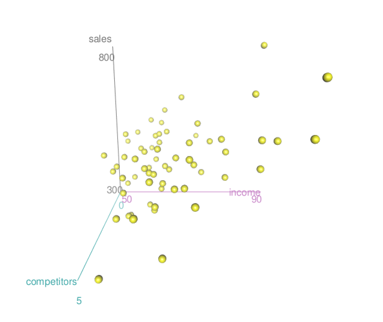
A retail company selling women's clothing has franchises across malls in America. It wants to investigate which factors are predictive of the number of sales per square foot of floor space (to level the playing field, since stores have varying footprints), and has collected annual data on $n=64$ of its stores. The company has a host of variables which it thinks may be predictive of sales. Two which we'll investigate:
Median income of the surrounding community (in thousands of dollars).
Number of competitor stores within the mall.
First: Visualizing Separate Regressions
> cor(sales, income)
[1] 0.6484524

(Intercept)       income
    120.458        6.081

> cor(sales, competitors)
[1] -0.05364514

(Intercept)  competitors
    517.434       -3.595

What are the Implications?
We saw that the correlation from the simple regression of sales on competitors seemed close to zero.
Does that mean that if I introduce a new competitor into a given mall, we won't expect that to have much of an effect?
Adding a Nordstrom won't affect Ann Taylor's sales?
All Together Now - Scatterplot Matrix
pairs(cbind(sales, income,
competitors))

cor(cbind(sales, income,
competitors))
        sales  income  compet.
sales    1.00   0.65   -0.05
income   0.65   1.00    0.40
compet. -0.05   0.40    1.00
All Together Now - Scatterplot Matrix
Malls with more competitor stores tend to be in more affluent areas! Higher income areas can support a larger number of similar stores.
So, in comparing two stores with different numbers of competitors based on our simple regression of
salesoncompetitors, we were also likely comparing stores in areas of varying affluence.
Fitting sales as a Multivariate Function
Intuitively, both competitors and income should matter. For a given store, we'd expect the sales to be a (noisy) function of both variables.
Through simple regression, we fit the functions:
$\widehat{\mathtt{sales}} = \hat{\beta}'_0 + \hat{\beta}'_1$
compet$\widehat{\mathtt{sales}} = \hat{\beta}''_0 + \hat{\beta}''_1$
income
What about a linear function of both variables?
\[ \widehat{\mathtt{sales}} = \hat{\beta}_0 + \hat{\beta}_1\texttt{compet} + \hat{\beta}_2\texttt{income} \]