STATS 413: Lecture 1
-
Introduction to linear regression
-
Simple regression
Regression Analysis
- Science and engineering
- Social Science
- Economics
- Finance
- Epidemiology
- Psychology and Education
- ...
Goals: use data to
-
to infer relationships between a single response variable and one or more other predictor variables.
-
to improve predictions of our response variable by leveraging information contained in the predictors.
Lexicon
In regression analysis, we seek to predict values of the ...
- Response Variable
- Dependent Variable
- Outcome Variable
- $y$ variable
Lexicon
...as a function of one or more...
- Predictor Variables
- Independent Variables
- $x$ variables
- Covariates
- Features
When performing a regression, we say that we regress the values of the $y$ variable on the values of the $x$ variables.
History
-
Sir Francis Galton, 19th century
Studied the relationship between heights of fathers and their sons and noted that the children "regressed" to the population mean -
Developed further by Yule, Pearson, Fisher in the late 1800s/early 1900s
-
Explosion in applied use with advent of modern computing in the 2nd half of the 20th century.
Questions to address with regression analysis
- point estimation: investigate quantitative questions about the parameters of a regression model
- Use data to come up with a prediction equation relating the response (e.g., height of a son) and the covariate(s) (e.g, height of the father).
- What is the slope of the line of best fit through the data?
Questions to address with regression analysis
- statistical inference: quantify uncertainty about our estimates, and assess what the data can tell us about population parameters
- How confident are we in our estimate of the slope? How much uncertainty is there? (confidence interval)
- Do taller fathers tend to have taller sons? (hypothesis test)
Questions to address with regression analysis
- prediction: predict the value of the response
- What's my best guess at the height of a son whose father is 73 inches tall?
- called supervised learning in machine learning
Regression Analysis
Goal: to infer population-level relationships between a response variable (denoted by $Y$) and one or more other explanatory variables (denoted by $X$) from data.
Data: values $(x_1,y_1),\dots,(x_n,y_n)$ of $(X,Y)$ observed on each of $n$ units or cases.
- $x_i\in\mathbf{R}^p$: predictors
- $y_i\in\mathbf{R}$: response variable
- $n$: sample size
Tabular Form
| Son.Height | Father.Height |
|---|---|
| 59.7 | 55.1 |
| 58.2 | 56.5 |
| ... | ... |
| 60.6 | 56.0 |
| 60.7 | 56.8 |
| 61.8 | 56.0 |
| 55.5 | 57.9 |
| 55.4 | 57.1 |
| 56.8 | 57.6 |
| ... | ... |
Data used for regression analysis is stored in tabular form, with a column for the response variable and one or more columns for the predictors
Data set: fatherson.csv. Contains height data for fathers and their sons.
General Tabular Form
If we have $p$ predictor variables along with our response...
| $y$ | $x_{1}$ | $x_{2}$ | $\cdots$ | $x_p$ |
|---|---|---|---|---|
| $y_{1}$ | $x_{1,1}$ | $x_{1,2}$ | $\cdots$ | $x_{1,p}$ |
| $y_2$ | $x_{2,1}$ | $x_{2,2}$ | $\cdots$ | $x_{2,p}$ |
| $\vdots$ | $\vdots$ | $\vdots$ | $\vdots$ | $\vdots$ |
| $y_n$ | $x_{n,1}$ | $x_{n,2}$ | $\cdots$ | $x_{n,p}$ |
Scatterplots
We use scatterplots for visualizing between two numerical variables
plot(father, son,...)
Linear Association
Informally, when saying that a relationship is linear, we mean that "The best description of the relationship between the two variables is drawing a line through the scatterplot."
-
The points in the scatterplot appear to be clustered about a line
-
Stronger relationship $\Rightarrow$ tighter cluster about the line
-
Positive and Negative relationships possible
Talking about a linear relationship makes sense if the point cloud is shaped like an ellipse
Scatterplots
There's a positive, linear relationship here.
-
Can we come up with a numerical measure describing the strength and direction of the linear relationship?
-
How do we exploit this relationship? We should be able to use a father's height to predict the height of his son by way of a linear equation.
Motivating Correlation
It would be nice to have a numerical measure of the strength/direction of a linear relationship. How should it behave?
-
Positive relationship $\Rightarrow$ Positive number; Negative relationship $\Rightarrow$ Negative number
-
Stronger relationships stand out numerically
-
Shouldn't depend on units
- Changing from feet to meters doesn't change the relationship!
Reminder: $z$-scores
For an observation $x_i$ of a variable $x$, the $z$-score of $x_i$, $z(x_i)$, answers the following question:
-
"How many standard deviations above (+) or below (-) the mean was the observed value $x_i$?"
-
Can write observation $x_i$ for the $i$-th individual as the mean, plus some number ($z(x_i)$) times the sd: $x_i= \bar{x} + z(x_i)\times \text{sd}(x)$. Solve for $z(x_i)$:
Reminder: $z$-scores
z-score
\[\textstyle z(x_i) \triangleq \frac{x_i - \bar{x}}{\text{sd}(x)}, \]
where
\[\textstyle \bar{x} = \frac{1}{n}\sum_{i=1}^nx_i;\quad\text{sd}(x) \triangleq(\frac{1}{n-1}\sum_{i=1}^n(x_i-\bar{x})^2)^{\frac12} \]Properties of $z$-scores
If we form $z$-scores of any continuous variable, $x$, then we have:
Mean, Standard Deviation of $Z$-Scores
\[ \begin{aligned} \text{mean}(z(x))&= 0\\ \text{sd}(z(x))&=1 \end{aligned} \]Properties of $z$-scores
Now, suppose I have a variable $x$, and I change units by $x^* = a + bx$:
Changing Units
If $b$ is positive, then $z(x^*) = z(x)$.
If $b$ is negative, then $z(x^*) = -z(x)$.
That is, the magnitude of $z$-scores are not affected by additive and multiplicative shifts (but the sign flips if $b$ negative)
Defining Correlation
Begin by taking $z$-scores of the $y$ and $x$ variables separately. Let $z(x_i) = \frac{x_i - \bar{x}}{\text{sd}(x)}$ denote the $z$-score of the $i$-th cases' $x$ variable value. Define $z(y_i)$ similarly.
Correlation Coefficient
\[ \begin{aligned} r(x,y) &\textstyle= \frac{1}{n-1}[z(x_1)z(y_1) + z(x_2)z(y_2) + \dots + z(x_n)z(y_n)]\\ &\textstyle= \frac{1}{n-1}\sum_{i=1}^nz(x_i)z(y_i) \end{aligned} \]Don't worry about the $n-1$...think of it instead as an average:
Defining Correlation
In English... Correlation is the mean of the products of the $z$-scores
Properties of Correlation
-
$-1\leq r(x,y) \leq 1$
-
Positive number implies positive relationship, negative number implies negative relationship
-
Unit free - consequence of taking product of $z$-scores.
- Changing units of $x$ or $y$ variable doesn't affect correlation!
-
Correlation between $X$ and $Y$ is equal to the correlation between $Y$ and $X$. $r(x,y) = r(y,x)$.
Properties of Correlation
-
Larger the value of $|r(x,y)|$, the stronger the linear relationship
-
$r(x,y) = 1$ implies points perfectly on a positive line, $r(x,y) = -1$ means points perfectly on a negative line
-
$r(x,y) = 0$ implies absence of a LINEAR association
Caveats about Correlation
-
Only tells us about overall linear relationship. Says nothing about nonlinear relationships
-
From the formula, we see it is dependent on both the mean and the standard deviation of the $x$ and $y$ variables. Hence, it can very easily by influenced by outliers
-
Correlation near zero doesn't mean there isn't a relationship, and furthermore it doesn't necessarily mean there isn't a linear relationship
-
Have to plot the data to check for outliers, and to check for a nonlinear relationship
Anscombe's Quartet
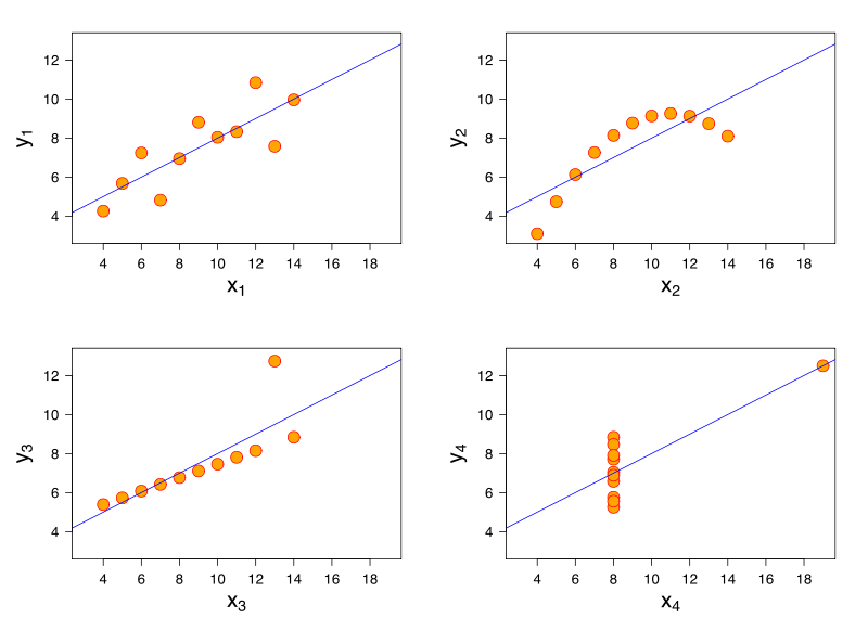
All have the same correlation! 0.816. VISUALIZE YOUR DATA
Enhancing Predictions
In our father's and son's height example: Suppose I pick an individual at random from the data set...
-
First, I simply ask you to guess what the son's height is, without giving you further information. What would your best guess be?
- The overall mean height
-
Instead, suppose I tell you the individual I selected had a father who was 74 inches tall (6'2"). Should we still guess that this individual's height is equal to the average height?
- Probably not... this individual is much taller than average! Should instead guess that this individual's son is taller than average too.
Heights of Fathers and Sons
As we'd expect, there's a positive linear association here. Tall fathers tend to have tall sons, short fathers tend to have short sons.
If I give you a father's height, what's your best prediction for his son's height?
One Reasonable (But Incorrect) Idea
What if we predict that the son's height will be as extreme as the father's height
-
Suppose we know a father's height is 75'' tall. The mean of father's height is 70.1'' with a sd of 2.5''
- $\Rightarrow$ Father has a $z$-score of roughly 2
-
The sons have an average height of 70.9 inches, with a sd of 2.4. If we predict the son to be as extreme, he should also have a $z$-score of roughly 2
-
$2 = \frac{y - 70.9}{2.4}\Rightarrow$ we should predict the son to have a height of 75.7''
Vertical Strips
-
Let's actually look at the data
-
On the scatter diagram, the points which have an $x$-value in common (at least approximately) make up a vertical strip of the data
-
They are color coded

The Average of the Vertical Strips
A good guess for the height of a son whose father is 75 inches is the average of the heights for all the sons whose fathers are (roughly) 75 inches. This is the AVERAGE inside a vertical strip
-
For this particular strip, the average son's height is 74 inches
-
The average of two of the vertical strips are marked: they roughly fall on a line! More on that later...

Which Approach is Right?
Earlier, I suggested that a good guess for the average height of the son would be 75.7'' (same $z$-score as father); now, I'm suggesting 74
-
Which is right? According to the actual data, 75.7 is usually way off
-
Again, sons overall have an average height of 70.9 in, with an SD of 2.4 inches.
- A son who is 74'' tall has a $z$-score of (74-70.9)/2.4 = 1.3, whereas the father had a $z$-score of roughly 2!
-
We are predicting the sons to be taller than average, but not as tall as their fathers on a relative scale ($z$-score of 1.3 vs 2)
On average, a son will regress towards the mean
The Regression Effect
Sir Francis Galton discovered this fact by staring at the scatter diagram of father's heights and sons's heights.
-
Observed that fathers who were tall had tall sons, and fathers who were short had short sons. This is due to correlation
-
Observed that fathers who were unusually tall/short had sons who were taller/shorter than average, just not as unusually tall/short on a relative ($z$-score) scale
-
The predicted heights were moving towards the mean. They were regressing!
The Regression Effect
Regression Effect
Given two correlated variables, if one variable is observed to be extreme, then you can expect the other variable to also be extreme—just not as extreme