Multilayer perceptrons
DATASCI 415: Statistical Learning and Data Mining
University of Michigan
including slides by Mu Li and Alex Smola
Multilayer perceptrons
(Multi-layer) Perceptrons
Multi-class classification
Optimization basics
Multi-class classification

Multi-class classification
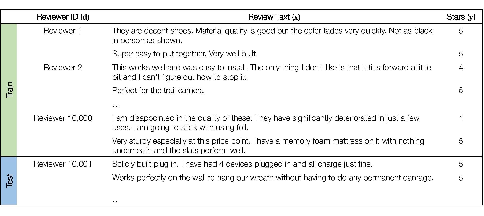
Regression vs $K$-class classification
regression outputs, predictions: (scalars) $y,\widehat{y}\in\reals$
($K$-class) classification
- outputs: one-hot encoding vectors $$e_k\triangleq\underset{1\text{ in }k\text{-th entry}}{[0\dots,0,1,0,\dots,0]}\in\{0,1\}^K$$
- predictions: $\widehat{y}$ are probability vectors; i.e. their entries are non-negative and sum to 1
outputs & predictions are probability distributions over the $K$-classes; i.e. they encode beliefs
- $y = e_k$: absolutely certain the example is from the $k$-th class
- $\widehat{y} = [\frac1K,\dots,\frac1K]$: uncertain which class the example is from
Regression vs $K$-class classification
regression loss: $\mathrm{SquareLoss}(y,\widehat{y})\triangleq(y-\widehat{y})^2$
($K$-class) classification loss:
$$\textstyle \mathrm{CrossEntropy}(y,\widehat{y})\triangleq -y^\top\log\widehat{y} = -\sum_{k=1}^K y_k\log\widehat{y}_k $$-
Unlike the square loss, the cross entropy loss is not symmetric; i.e.
$$\mathrm{CrossEntropy}(y_1,y_2) \ne \mathrm{CrossEntropy}(y_2,y_1).$$ -
If $y$ is a one-hot encoding, then $\mathrm{CrossEntropy}(e_k,\widehat{y}) = -\log\widehat{y}_k$. Thus the cross entropy loss is also called the log loss.
Regression vs $K$-class classification
regression training: $\min_wL(w)$
$$\begin{aligned} L(w) &\textstyle= \frac1n\sum_{i=1}^n\mathrm{SquareLoss}(y_i,f(x_i;w)) \\ &\textstyle= \frac1n\sum_{i=1}^n(y_i-f(x_i;w))^2 \end{aligned}$$(multi-class) classifier training: $\min_wL(w)$
$$\begin{aligned} L(w) &\textstyle= \frac1n\sum_{i=1}^n\mathrm{CrossEntropy}(y_i,f(x_i;w)) \\ &\textstyle=-\frac1n\sum_{i=1}^ny_i^\top\log f(x_i;w) \end{aligned}$$If the $i$-th example is from the $k$-th class, then $$\mathrm{CrossEntropy}(y_i,f(x_i))= -\log f_k(x_i;w),$$ so cross-entropy minimization "pushes" $f_k(x_i;w)$ towards 1.
NN for multi-class classification
MLP with 1 hidden layer:
$$\begin{aligned} h^{(1)} &\gets \sigma(W^{(1)}x + b^{(1)}) \\ o &\gets (w^{(2)})^\top h^{(1)} + b^{(2)} \end{aligned}$$
- exponentiate to obtain positive numbers
- divide by the sum to obtain a probability distribution
NN for multi-class classification
MLP with L hidden layers:
$$\begin{aligned} h^{(1)} &\gets \sigma(W^{(1)}x + b^{(1)}) \\ &\;\;\vdots \\ h^{(L)} &\gets \sigma(W^{(L)}h^{(L-1)} + b^{(L)}) \\ o &\gets (w^{(L+1)})^\top h^{(L)} + b^{(L+1)} \end{aligned}$$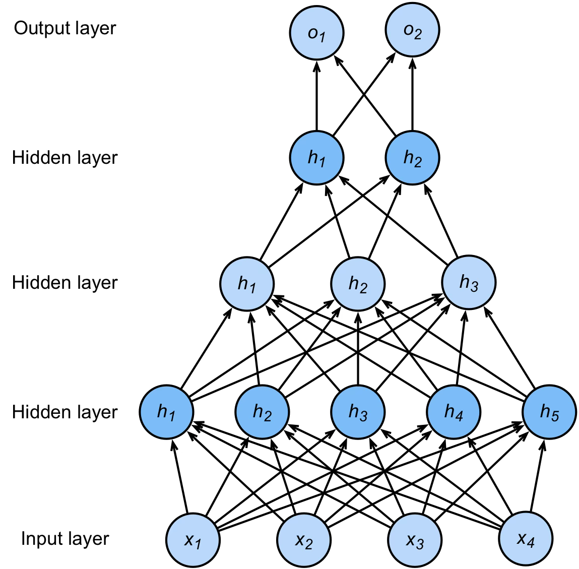
Gradient descent
$$\textstyle\min_w L(w)$$- $L$ is the training loss
- $w$ is a vector of parameters (e.g. NN weights)
Inputs
- learning rate schedule/sequence $(\eta_t)_{t=1}^\infty > 0$
- starting point $w_0$
Loop
- compute gradient $\nabla L(w)$
- update $w_{t+1}\gets w_t - \eta_t\nabla L(w_t)$
until converged
Gradient descent
$$\textstyle\min_w L(w)$$- $L$ is the training loss
- $w$ is a vector of parameters (e.g. NN weights)
Loop
- compute gradient $\nabla L(w)$
- update $w_{t+1}\gets w_t - \eta_t\nabla L(w_t)$
until converged
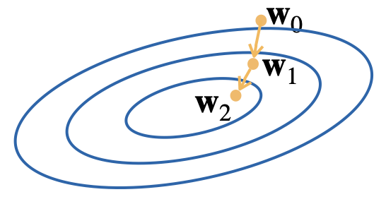
Choosing learning rates
learning rate too small
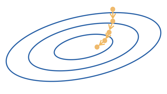
learning rate too big
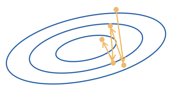
Gradient descent is guaranteed to converge to a (local) minimum as long as the learning rates are small enough.
Stochastic gradient descent (SGD)
The training loss is an average over training examples:
$$\textstyle L(w) = \frac1n\sum_{i=1}^n\ell_i(w),\quad\ell_i(w)\triangleq\ell(y_i,f(x_i;w)).$$Computing $\nabla L(w)$ can be costly (taking hours or even days) because it entails making a pass over all training examples:
$$\textstyle\nabla L(w) = \frac1n\sum_{i=1}^n\nabla\ell_i(w).$$Idea: approximate $\nabla L(w)$ with a random batch of training examples
$$\textstyle \frac{1}{|\cB|}\sum_{i\in\cB}\nabla\ell_i(w)\approx \nabla L(w)$$Stochastic gradient descent (SGD)
Loop
- randomly select $\cB\subset[n]$
- approximate gradient $g_t\gets\frac{1}{|\cB|}\sum_{i\in\cB}\nabla\ell_i(w)$
- update $w_{t+1}\gets w_t - \eta_t\nabla L(w_t)$
until converged

The batch size is an important hyperparameter
- batch size too small: slow convergence
- batch size too big: wasted computation