


Differences between kinds of political action committees (PACs) allow us indirectly to observe variations between presidential and midterm election periods in one of the two variables that are chosen in the first stage of the game model and that determine the type of dynamics that occur in system (1). The variable is challenger quality (h). We can therefore formulate predictions about differences that ought to be observed in the qualitative character of the dynamics in moving from one election period to the other. I use these predictions to motivate statistical tests of the key qualitative properties of the formal theory, using data from the 1984 and 1986 election periods.
Challenger quality ought to vary systematically between election years. In
terms of vote share, the President's party invariably lost support in midterm
congressional elections from 1918 through 1990 (Alesina and Rosenthal 1995,
84). But if the chances that an opposition party candidate will win the
general election are reliably higher in the midterm year, then Banks and
Kiewiet's (1989) analysis that shows that challengers ought to run when their
chances of winning are greatest implies that challengers not of the
president's party ought to be of higher quality at midterm than during the
presidential election year. Banks and Kiewiet's argument further suggests
that higher quality opposition party challengers ought to have an easier time
of it during the primary season, as the expectation that the higher quality
challengers will enter ought to deter lower quality opposition party
challengers from entering. A similar argument suggests that challengers of
the same party as the President ought to be of higher quality during the
presidential election year than at midterm.
Challenger quality also ought to vary systematically across kinds of PACs.
Due to the respective parties' policy positions, labor PACs during the 1980s
tended to favor Democratic incumbents (Grier and Munger 1986; Endersby and
Munger 1992) and challengers (McCarty and Poole 1998). Corporate PACs tended
to have been biased in favor of Republican incumbents (Grier and Munger
1986) and challengers
(McCarty and Poole 1998). Due to the conservative ideological bent of many
high-profile non-connected PACs throughout the 1980s (Latus 1984),
non-connected PACs tended to be biased in favor of Republican candidates
during the 1984 and 1986 election cycles (McCarty and Poole 1998). Given the
Republican presidential victory in 1984 and challengers' likely reactions to
the midterm loss phenomenon, it follows that the Democratic challengers that
labor PACs typically preferred to support ought to have increased in quality
from 1984 to 1986, while the more Republican mix of challengers that corporate
and non-connected PACs favored ought to have decreased in quality.
According to the theory that leads to Figure 3, such systematic variations in challenger quality across years and across PACs ought to imply corresponding variations in the stability of campaign dynamics. For labor PACs, from the 1984 to the 1986 campaign periods there ought to be movement up the challenger quality axis of the bifurcation diagram of Figure 3. The dynamics for labor PACs ought therefore appear more stable during the 1984 period than during the 1986 period. For corporate PACs and non-connected PACs, from 1984 to 1986 there ought to be movement down the challenger quality axis. The dynamics for corporate and non-connected PACs ought therefore appear less stable during the 1984 period than during the 1986 period.
I use two tests to evaluate whether the stability of the dynamics changes as
predicted between election periods. The distance test assesses
whether the 4DH model's estimated origin for the dynamics,
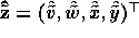 , is farther from the sample mean
(
 ) of the observed data
 during the election period for which more unstable
dynamics are predicted than it is during the period for which more stable
dynamics are expected. The greater the distance between
 and , the more likely it is that
the dynamics are occurring in region II of Figure 3, where the fixed
points are a spiral source and a saddle point, rather than in Figure 3's
regions I (spiral sink) or III (limit cycle). As I explain in the Appendix,
under the null hypothesis of no difference in stability between election
periods, the test statistic for the distance test has a doubly noncentral
F-distribution.
The second test, the divergence test, checks for a geometric feature
that distinguishes stable from unstable dynamics. Stable dynamics push flows
closer together, while unstable dynamics spread flows farther apart. The rate
at which flows in a vector field  tend in this way either to increase or
to reduce the volume of a bounded set can be measured by integrating the
divergence of the vector field, denoted
 , over the interior of the
set. To estimate the divergence for the observed data I use vectors
 to estimate the vector field. The set of vectors
 is computed by plugging the parameter estimates into model
(3) and then evaluating the resulting equations for each observed
data point. The divergence estimate is
 . The
divergence test is a one-tailed t-test for the equality of the sample means
of
 between election periods. The mean divergence
should be greater for the period predicted to be more unstable. The Appendix
gives a more complete explanation of the divergence test.
I estimate the 4DH model by maximum likelihood with district-level data for
the U.S. House elections of years 1984 and 1986. The observed variables correspond to the formal variables of
system (1) that were used in Figure 2 to illustrate the
system's flows. Variable  represents
post-election district service, measured by intergovernmental transfers from
the federal government to local governments in each congressional district
during the year following each election: I use 1985 transfers for the
1984 election period and 1987 transfers for the 1986 election period.
Intergovernmental transfers are a kind of district service that Members of
Congress are well-known to affect (Arnold 1979; Haider 1974; Stein and Bickers
1995). I consider separately four types of transfers: education transfers;
highways transfers; social welfare transfers; and other transfers.
is the natural logarithm of the amount originally measured in
units of $1000 per person.
Variable
 represents incumbent contributions, measured by the
total amount of PAC campaign contributions to each incumbent during each
two-year campaign period. Variable
 measures the total of all
such contributions given to any challengers in each district. I consider
separately contributions from corporate PACs, labor PACs and non-connected
PACs (Federal Election Commission 1984-88). and
are the natural logarithms of amounts originally measured in units of $1 per
person, based on district population (Bureau of the Census 1983; 1986).
Variable
 , where P is the proportion of all
general election votes cast for the incumbent (Scammon and McGillivray 1983;
1985), represents the probability p that the incumbent wins. While
 , p ought to be stochastically increasing in P.
The test results, in Table 3, give extremely strong support to
the qualitative hypotheses. In every instance, both the distance test and the
divergence test indicate that for corporate and non-connected PACs the
dynamics are less stable during the 1984 election period than during the 1986
election period. For labor PACs, the distance test does not indicate any
significant increases between 1984 to 1986 in the separation between
and . But for all four types
of spending the divergence test indicates that the 1986 dynamics for labor
PACs are significantly less stable than the dynamics of the 1984 period.
The estimated vector fields plotted in Figures 4 and
5 illustrate the kinds of changes in the dynamics that
the distance test is measuring.
For each district i that has observed data  , a vector is
represented by an arrow that has base at and head at
 . Each Figure shows the vector field for four observed
variables--post-election intergovernmental transfers for highways ( ),
corporate PAC contributions to the incumbent ( ) and to challengers
( ), and incumbent vote share (
 )--projected into one subfigure for
each pairing of the variables. In each subfigure a circle marks the estimated
origin, i.e., the appropriate pair of the estimates
 ,
 ,
 and
 .
Figure 4 shows estimates for the 1984 election period and
Figure 5 shows estimates for the 1986 election period. It is
easy to see that the dynamics are much more unstable in 1984 than in 1986. In
the three subfigures of Figure 4 that project the vector field
into the planes defined by the post-election transfers and each of the other
three variables, the estimated origin is clearly at
a remove from the bulk of the data. There is no such pattern in
Figure 5. In Figure 5 most of the vectors seem
to be pointing inward, toward the centrally located origin.
For corporate and non-connected PACs, the formal test results and estimated vector fields such as those shown in Figures 4 and 5 strongly suggest that during the 1984 election period there are unstable dynamics like those in region II of Figure 3's bifurcation diagram, but that during the 1986 period there are stable dynamics like the spiral sinks of Figure 3's region I. Vector field estimates for labor PACs (not shown) do not suggest a qualitative change between 1984 and 1986, but the divergence test strongly indicates that some kind of change does occur. The dynamics involving labor PACs during the 1986 election period are more unstable than the dynamics during the 1984 election period, but it is unlikely that the dynamics are as unstable as those in Figure 3's region II.
According to the theory that leads to Figure 3, the simplest explanations for the differing patterns of change are two. One possibility is that all three types of PACs are interested in the same type of service from the winner of the election, but somehow the challengers that corporate and non-connected PACs support during the 1984 election period are of higher quality than the challengers that labor PACs support during the 1986 election period. In this case, in Figure 3, the service type (g) would have roughly the same value for all three types of PACs, but the greater quality (h) of the challengers that the corporate and non-connected PACs support in 1984 would place them further up the h axis. The greater h values would induce dynamics that are substantially more unstable than those induced by the challengers that labor PACs supported in 1986.
The other simple possibility is that there is not much difference across types
of PACs in the range of challengers' quality. Rather labor PACs may be
interested in types of service that provide benefits that are more
concentrated than the benefits that motivate corporate and non-connected PACs.
The idea is that such a difference in the type of service may place the
dynamics for labor PACs to the right of the Cournot-Nash equilibrium point in
Figure 3 (i.e.,  ), while putting the dynamics for
corporate and non-connected PACs to the left of that point (
 ).
Then an increase in challenger quality capable of shifting the dynamics for
corporate and non-connected PACs from region I into region II may not be
sufficient to move the dynamics for labor PACs out of region I. The
divergence of the vector field for labor PACs would increase, but the
qualitative character of the dynamic equilibrium point would not change. It
would remain a sink, with flows tending to spiral in on it.
Are the benefits that labor PACs seek more concentrated than the subsidies, tax exemptions, regulatory changes and special legislation that most often interest the sponsors of corporate or non-connected PACs? Presumably labor PACs focus on the interests of their sponsoring union memberships. The current data are not sufficient to pursue this question, but the possibility is an intriguing and surprising suggestion from the analysis. Whatever the correct answer to the question may be, the way that it comes to the forefront here helps demonstrate the depth of substantive insight that can be supported by the 4DH model's ability to recover information about dynamics from cross-sectional data.