


To estimate the relationships between LFE levels and support across geographic
areas we estimate equation (2) separately for each of sixteen
different kinds of LFEs, using annual, county-level data for years
1985-88. The specification is designed to check whether LFE targeting
behavior varies during the President's term. We focus on the distinction between
targeting early and targeting late in the term, using the midterm election as
the dividing point.
To measure the President's information  we use two different
quantities. During the first two years of the term, we measure information by
the proportion of the two-party vote cast for the incumbent in each county in
the preceding presidential election, transformed using the inverse Normal CDF.
I.e., during the first two years,
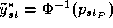 , where
 denotes the preceding vote proportion in county s.
During the second two years, we use ANES data to simulate the support the
President might expect to receive at midterm from each county if individual
voters were to use at that time the same voting decision rule they used in the
preceding election. This approach gives post-midterm information values
computed using
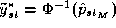 , with
where  is the predicted probability that voter i surveyed
in the midterm ANES would vote for the President, and
 is the
number and
 is the set of all voters in the midterm sample in
county s. Details regarding the computation of the probabilities
appear in the Appendix.
We use polynomials to approximate the targeting functions  . That
is, for each kind of LFE we define
 , for constant
coefficients
 and some choice of polynomial degree m (this
gives Appendix equation (4)). To choose m we use F-tests
based on deviance statistics.
The variables  include a set of dummy variables that represent
the annual memberships on fifteen standing committees of the U.S. House
delegation from the State to which county s belongs, and a variable that
measures the annual average for the State of the number of consecutive terms
served by the State's House members. We use these variables
to measure congressional influence on LFEs.
The sixteen LFEs cover most federal expenditures that disburse funds in particular geographic areas in the United States. The LFE variables include transfer payments, civilian and military employment, salaries and procurements, direct payments (not for individuals and not procurements) and intergovernmental transfers to local governments for education, for highways, for social welfare or for other purposes. The LFE variables are listed, with source citations, in Table 1. For the LFE variables that measure money the values are the total dollar amount spent in each county in each year, divided by the county population in that year; units are $1000 per person. For the variables that measure employment, the values are the total number of jobs, per capita, with units being jobs per person. In light of the fact that many Federal grants that are ultimately disbursed by local governments are passed through State governments, we analyze, separately, transfers to local governments from State governments as well as from the Federal government.
The estimated targeting function polynomials are plotted in Figures
1 and 2. The values represent partial LFE levels (net
of congressional influences and fixed effects), plotted against the support
scores and  . The ranges of values for
and used in the figures are the values that
occur for the counties in the ANES data. Figure 1 shows the
pre-midterm polynomials and Figure 2 shows the post-midterm
polynomials. Table 2 shows the 95% confidence interval for the
local maximum of each curve on the [0,1] interval, when such exists.
The estimates suggest that targeting was induced by patronage delegation for more than half of the kinds of LFEs. Recall that for elite-induced targeting we expect to see the most spending in local areas where the President received about 50-70% of the votes. Because local elites newly appointed after the election will immediately commence trying to deliver benefits to the areas they came from, this pattern ought to be most apparent during the first part of the President's term. The figures and Table 2 clearly show the expected pattern during the pre-midterm period for seven kinds of LFEs: civilian procurements, military employment, civilian salaries, Federal social welfare and education transfers, and State highways and education transfers. The other LFEs do not show the expected pre-midterm pattern. Only one LFE--civilian procurements--shows the expected pattern during the post-midterm period.
To check for voter-oriented targeting we need to measure the changes that
occur over time in each kind of LFE as a function of the President's support
in each local area. We use the targeting polynomial estimates for this
purpose by computing the difference between the predicted post-midterm and
pre-midterm levels of each LFE in the idealized case where the President's
support remains constant at some level throughout the term. I.e., we compute
the difference 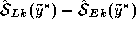 for a range of
 values. For voter-oriented targeting we expect to
see the largest increases in spending for support values between roughly .3
and .5
The simulated differences plotted in Figure 3 and 95% confidence
intervals for local maxima shown in Table 3 suggest that
voter-oriented targeting occurred for about half of the LFEs we rated as
relatively low in institutional complexity but occurred for at most one of the
LFEs we rated as high in institutional complexity. The simulated differences
for military employment, civilian and military salaries and transfer payments
all have maxima near  . For military salaries and transfer
payments these are the global maximum points. The exceptional pattern among
institutionally complex LFEs occurs for Federal social welfare transfers; the
polynomial has a local maximum near
 but achieves higher
values as increases above
 .
