Shear and Loading in Channels: Oscillatory Shearing and Leapfrogging Edge
Currents of Fluxons in Superconductors
J.F. Wambaugh1,
F.
Marchesoni1,2, and
Franco
Nori1*
1. Department
of Physics, University of Michigan, Ann Arbor, Michigan 48109-1120
2. Istituto Nazionale di Fisica della
Materia, Universit'a di Camerino, Camerino, I-62032, Italy
We study via computer simulations the motion of magnetic flux-line
vortices (fluxons) confined to a straight pin-free channel in a strong-pinning
superconducting sample. We find that, when a constant current is
applied across this system, a very unusual oscillatory shearing manifests,
in which the fluxons at the edges of the channel repeatedly trail behind
and then suddenly leapfrog past the inner rows. For small enough
driving forces, the oscillatory shearing dynamic phase is replaced by a
continuous shearing phase in which the distance between initially-nearby
fluxons grows in time, quickly destroying the order of the lattice.
 Simulation
---
Unless
otherwise specified, each figure refers to simulations conducted in the
following way: Initially fluxons were placed uniformly across the
sample in a minimum-energy, field-cooled triangular lattice and the fluxons
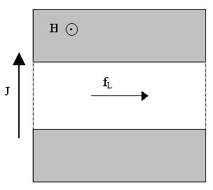
in the channel were subjected to a current along y; producing a
Lorentz driving force F º fL
/ f0 = 15. The square sample had side 18 l
and the central straight channel was parallel to the x-axis, centered
in the sample and 7 l wide. This configuration
is schematically depicted in Fig. 1. The initial triangular distribution
resulted in roughly two thirds of the fluxons being fixed in the very strong
pinning region outside the central channel. The square sample had
periodic boundary conditions, allowing free fluxons in the channel to continue
moving along the x-axis indefinitely. Because of the channel
walls, periodic boundary conditions along the y-axis did not affect
the dynamics. Typically Dt = .01 was used.
giving the unit of time t = 100 MD steps.
Simulation
---
Unless
otherwise specified, each figure refers to simulations conducted in the
following way: Initially fluxons were placed uniformly across the
sample in a minimum-energy, field-cooled triangular lattice and the fluxons
in the channel were subjected to a current along y; producing a
Lorentz driving force F º fL
/ f0 = 15. The square sample had side 18 l
and the central straight channel was parallel to the x-axis, centered
in the sample and 7 l wide. This configuration
is schematically depicted in Fig. 1. The initial triangular distribution
resulted in roughly two thirds of the fluxons being fixed in the very strong
pinning region outside the central channel. The square sample had
periodic boundary conditions, allowing free fluxons in the channel to continue
moving along the x-axis indefinitely. Because of the channel
walls, periodic boundary conditions along the y-axis did not affect
the dynamics. Typically Dt = .01 was used.
giving the unit of time t = 100 MD steps.
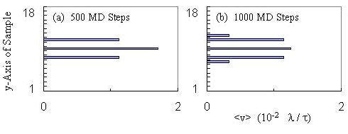
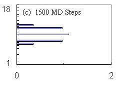
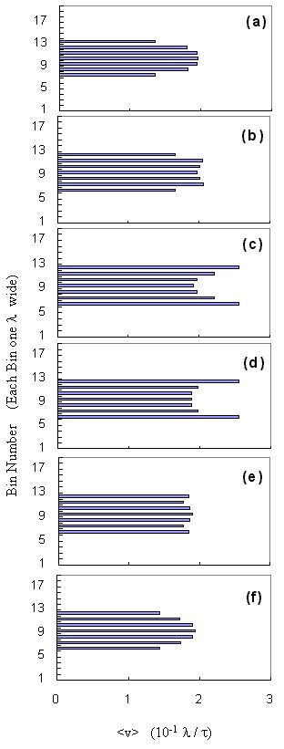
Fluxon Velocities inside the Channel --- Figure 2 shows
a "velocity profile" computed by dividing the sample into 1 l
wide, horizontal "bins" and averaging the velocity of those fluxons in
each bin.
We want to monitor the time evolution of v(y), since shear
implies a non-zero gradient along y of v(y).
We have found that binned velocity snapshots, like the ones shown in Fig.
2, are useful because they illustrate the shear-induced presence of gradients
in v(y). Thus, we binned the fluxon velocity along
y
and integrated the velocities along x.
The two sequences [(a--c) and (d--f) in Fig.~2] of velocity profiles
across a channel are successive velocity snapshots. These snapshots
are made every 500 MD steps during the course of a simulation: (a--c) shows
three successive snapshots, while in (e--f) every third snapshot is shown.
These two particular chronological sequences show two different types of
behaviors that we have found when a perfect triangular lattice of fluxons
is placed and then forced to move on a superconducting sample with a straight
channel.
Continously Sheared Dynamic Phase for Low Driving
Sequence (a--c) in Fig. 2 corresponds to a relatively weak driving force
of magnitude F = 0.02, and displays the expected "beer-belly" curved velocity
profile. Here the shear between the edge fluxons of the channel and
the pinned fluxons outside the channel induces a curvature in the velocity
profile. In (a), the edge rows, interacting with the infinitely pinned
fluxons experience drag, resulting in the inner row moving slightly faster.
The interaction between the inner (bin 9) and outer (bins 7 and 11) fluxon
rows pulls the outer rows along, eventually pushing outwards a few fluxons
in the edge rows---as they catch on the pinned fluxon potential, as shown
in (b). This outward displacement of a few edge fluxons creates defects
in the moving fluxon lattice and also the appearance, in the velocity profile
in (b), of moving fluxons (in bins 6 and 12) where there were previously
none. For this low density of fluxons, and for our chosen fine-grained
bins, there are no fluxons in bins 8 and 10. A higher density example
will be discussed below. In (c), the velocity profile has remained
"fanned out" as the fluxons continue to be driven. The original triangular
lattice arrangement has not been preserved because the fluxon lattice has
been continuously sheared, producing many defects. Indeed, the distance
between initially nearby fluxons grows with time, for low driving forces.
Oscillatory Shearing Dynamic Phase for Higher Driving
At a higher driving force, however, a novel dynamic fluxon phase is
observed. Sequence (d--f) in Fig. 2 has the same number of fluxons
as in (a--c), but driven by a higher driving force; F = 1 instead of F
= 0.02. Now, instead of allowing fluxons to slip from the outer rows
as they catch on the interactions with pinned fluxons, the outer rows of
fluxons actually leapfrog forward past the inner row, by temporarily
moving more rapidly than the inner row. Here, (e) clearly shows the
outer rows actually move faster than the inner rows. Eventually,
the faster edge rows slow down and, as shown in (f), this results in a
brief effective uniform velocity across the channel.
This unexpected cycle repeats periodically and it is even more pronounced
when there are higher fluxon densities, corresponding to higher magnetic
fields. The three-row arrangement shown here is just the simplest
example that illustrates this novel fluxon dynamic phase.
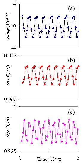 Further
Characterization --- Figure 3 shows the temporal evolution of the
difference in velocities vdiff between the inner and
outer rows (a). The overall average velocity in the channel has also
been plotted, in (b) to show how vdiff correlates to
v.
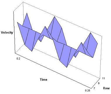
The velocity in (b) changes to (c) when the number of vortices is increased
from 80 to 340. Below is a contour giving the evolution of velocity
across the channel with time.
Further
Characterization --- Figure 3 shows the temporal evolution of the
difference in velocities vdiff between the inner and
outer rows (a). The overall average velocity in the channel has also
been plotted, in (b) to show how vdiff correlates to
v.
The velocity in (b) changes to (c) when the number of vortices is increased
from 80 to 340. Below is a contour giving the evolution of velocity
across the channel with time.
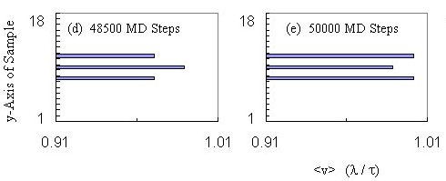
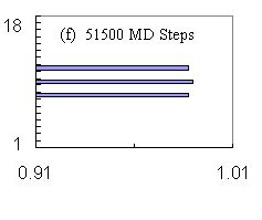
 Leapfrogging
Edge Fluxons at Higher Fluxon Densities --- The very unusual cycle
of "trail-behind" and leapfrogging edge fluxons seen in Fig. 2 very clearly
persists at much higher field strengths, as indicated in Fig. 4.
There, the density of fluxons is about four times higher than in the case
shown in Fig. 2.
Leapfrogging
Edge Fluxons at Higher Fluxon Densities --- The very unusual cycle
of "trail-behind" and leapfrogging edge fluxons seen in Fig. 2 very clearly
persists at much higher field strengths, as indicated in Fig. 4.
There, the density of fluxons is about four times higher than in the case
shown in Fig. 2.
The chronological sequence of "snapshots" in velocity space in Fig.
4 depicts the time evolution of the velocity of fluxons across the channel.
This situation is similar to Fig. 2 (d--f), but now there is a much higher
field strength: 340 fluxons have now been placed in a triangular lattice
on the sample with a straight central channel. This combination of
field strength and channel width results in the channel being filled with
seven horizontal rows of seventeen fluxons each.
The behavior exhibited in Fig. 4 is the result of inner rows of fluxons
being locked together with the outer rows despite the interactions of the
outer rows with the pinned fluxons outside the zero-pinning channel.
Intuitively one would expect that profiles like (a), (b) and (f) are the
norm---the outer rows snag on the pinned fluxons and lag behind the less
restricted inner rows. The surprising behavior is that profiles like
(c) and (d) indicate that the slowed fluxons in the outer rows suddenly
"catch up" or leapfrog by momentarily exceeding the velocity of
fluxons in the inner rows. Panel (e) in Fig. 4 shows that this can
also result in a much flatter velocity profile than otherwise expected,
albeit just briefly.
Simulations at both field strengths discussed here (80 and 340 fluxons
on the sample) demonstrate continuous shearing under low driving forces,
but unusual oscillatory shearing under higher driving forces. In
addition to higher field strengths, simulations with smaller Dt's
were used, producing the same results (e.g., 0.001 instead of 0.01).
The animation shows the change in velocity profile during a simulation
with smaller Dt (the velocities are larger than
those in the snapshots because the particular simulation animated was conducted
with F = 1 instead of F = .2 as in the snapshots).
 Velocity
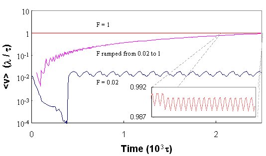
versus Time for Several Driving Forces --- Figure 5 shows the fluxon
velocity, now averaged over the entire sample, for the oscillating
shearing phase (top curve, F = 1), the continuous shearing phase (bottom
curve, F = 0.02), and an intermediate ``ramped driving" case, where the
driving force is slowly increased to monitor the crossover (not
a sharp dynamic phase transition) between these two dynamic phases.
Several simulations were done, but only three representative ones are shown
here.
Velocity
versus Time for Several Driving Forces --- Figure 5 shows the fluxon
velocity, now averaged over the entire sample, for the oscillating
shearing phase (top curve, F = 1), the continuous shearing phase (bottom
curve, F = 0.02), and an intermediate ``ramped driving" case, where the
driving force is slowly increased to monitor the crossover (not
a sharp dynamic phase transition) between these two dynamic phases.
Several simulations were done, but only three representative ones are shown
here.
The lowest curve shown in Fig. 5 corresponds to a weak-driving case;
here with force F = 0.02. First, there is a transient. Afterwards,
the average velocity of the entire lattice, not just the edge fluxons anymore,
shows marked oscillations with time. This corresponds to a "stick-slip"-type
motion of the fluxon lattice impinging upon a succession of potential
energy bottlenecks as it is pushed through the channel. Notice
that strictly speaking, the "stick" phase is really moving, and never stuck.
Thus, it is more appropriate to describe it as a phase with an oscillating
sine-like average velocity. Notice also that the velocity oscillations
in this low-driving "continuous shearing" dynamic phase span about 1/3
of an order of magnitude (the vertical axis has a logarithmic scale).
The highest curve in Fig. 5 shows a typical large-driving, F = 1, case.
There, the system is in the oscillating shearing dynamic phase, and the
average velocity of the entire system oscillates, as shown in the magnification
of this plot located in the lower right inset. The average velocity
appears to be constant in the main panel of Fig. 5 because its vertical
axis spans five decades!
To monitor the crossover between these two dynamic phases, Fig. 5 also
shows an intermediate curve, where the driving force was slowly increased
from an initial value of F = 0.02 to a final value of F = 1.
While the average velocity oscillations of the continuous shearing phase,
the low-driving-force-regime, initially persist, it is clear that the amplitude
of the velocity oscillations decrease until there is no discernable oscillation
(without magnification) in the logarithmic plot.
In other words, when the average velocity of the moving fluxons is plotted
over time, while the driving force is slowly increased, the average velocity
eventually becomes relatively stable, in the sense that there is not much
overall relative shifting in the lattice. Thus, the lattice, while
sheared with oscillating velocities,
is not completely torn apart at higher driving forces---because of
the periodic "leapfrog" jumps of the trailing edge fluxons.
For the measurements shown in Fig. 5, the average displacement of all
moving fluxons was recorded every 500 MD steps, over the course of 250,000
MD step simulations. We also studied many more values for the driving
force, including very high values. For all cases where F was approximately
larger than 0.05, oscillating shearing was found.
Since the oscillations in the average velocity are caused by the interaction
between the moving and pinned fluxons, we have found that the frequency
of the oscillations depends on the density of the fluxons (they are inversely
proportional). Thus, careful measurements of the average velocity
(e.g., as a voltage), might provide an indirect way of determining the
fluxon density and magnetic field strength. Indeed, in Fig. 3, the
system that produces the signal (c) is the same one as in (b) but with
about four times the number of vortices. Notice how the period decreases.
* Corresponding author.