In the previous sections we have assumed that there were no radial variations in velocity, concentration, temperature or reaction rate in the tubular and packed bed reactors. As a result the axial profiles could be determined using an ordinary differential equation (ODE) solver. In this section we will consider the case where we have both axial and radial variations in the system variables in which case will require a partial differential (PDE) solver. A PDE solver such as COMSOL Multiphysics, will allow us to solve tubular reactor problems for both the axial and radial profiles.
Figure P8-24a Shell balance.
In order to derive the governing equations we need to add a couple of definitions. The first is the molar flux of Species A, WA mol/m2•s. The molar flux has two components, the radial component WAr, and the axial component, WAz. The molar flow rates are just the product of the molar fluxes and the cross sectional areas normal to their direction of flow Acz. E.g. for species A
FAz= WAz Acz
where Acz is the cross sectional area of the tubular reactor.
In
chapter 11 we discuss the molar fluxes in some detail, but for now let us just say they consist of a diffusional
component,
![]() , and a convective flow component,
, and a convective flow component,
![]()
![]()
where De is the effective diffusivity m2/s, and Uz is the axial molar average velocity, (m/s). Similarly the flux in the radial direction is
![]()
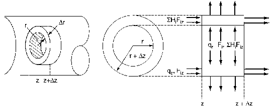
where Ur is the molar average velocity in the radial direction. A mole balance on a cylindrical system volume of length Dz and thickness Dr gives
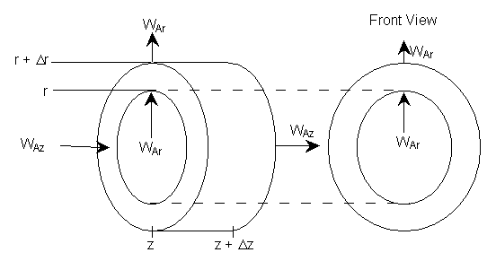
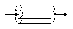
Figure 8-4 Cylindrical shell of thickness Dr and length Dz
![]()
![]()
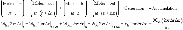
Dividing by 2prDrDz and taking the limit as Dr and Dz ® 0
![]()
Similarly for any species i
![]() (8-X)
(8-X)
Substituting for Wiz and Wir
![]()
Assumption 1. Ur is essentially zero.
![]()
Assumption 2. Uz is constant wrt z.*
![]()
*1F Uz is not constant then we have another
term
![]() , with
, with
![]()
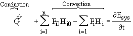
When we applied the first law of thermodynamics to a reactor to relate either temperature and conversion or molar flow rates and concentration, we arrived at Equation (8-9). Neglecting the work term we have
The
![]() term is the heat added to the system most always includes a conduction component of
some form. Neglecting PV work, the total energy of the system
term is the heat added to the system most always includes a conduction component of
some form. Neglecting PV work, the total energy of the system
![]()
We now define an energy flux, e, (J/m2•s).
![]()
![]()
where q
![]() is given by Fourier's law. For axial conduction Fourier's law is
is given by Fourier's law. For axial conduction Fourier's law is
![]()
where kc is the thermal conductivity (J/m•s•K). The energy transfer (flow) is the flux times the cross sectional area, Ac, normal to the energy flux
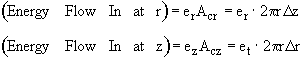
Energy flow = e • Ac
Energy Balance
Using the energy flux, e, to carry out an energy balance on our system volume 2prDrDz we have
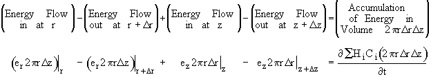
![]()
Dividing by 2prDrDz and taking the limit as Dr and Dz ® 0
![]()
![]()
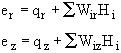
Substituting for e
![]()
and expanding the convective energy flux,
![]() ,
,
![]()
we obtain

Recognizing the term in brackets is related to Eqn (8-X) and is just the rate of disappearance of species i, -ri. We have
![]()
Recalling
![]()
and
![]()
we have

![]()
Assumption 3. The diffusive flux,
![]() , in the radial direction is greater than the convective flux, i.e.
, in the radial direction is greater than the convective flux, i.e.
![]() , thus
, thus
![]()
Assumption 4. The convective flux in the axial direction,
UCi, is greater than the diffusive flux,
![]() , consequently the flux of species i in the axial direction is
, consequently the flux of species i in the axial direction is
![]()
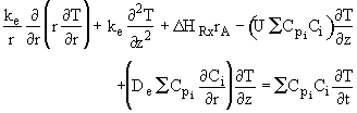
With these approximations we have

Assumption 5. Neglect the convective energy flux in the radial direction
![]() with respect to the conductive flux,
with respect to the conductive flux,
![]() . The energy balance now becomes
. The energy balance now becomes
![]()
where
![]() and is assumed constant.
and is assumed constant.
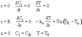
A. Initial conditions
![]()
B. Boundary condition
(1) Radial
(a) At
r = 0, we have symmetry
![]()
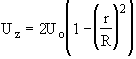
(b) At the tube wall r = R, the flux to the wall on the reaction side equals the convective flux out of the reactor into the shell side of the heat exchanger.
![]() with
with
![]()
(c)
There is now flow through the tube walls
![]()
(d) At the entrance to the reactor z = 0
![]()
(e) at the exit of the reactor
z = L
![]()
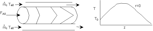
The following examples will solve the above equation using COMSOL Multiphysics. For the exothermic reaction with cooling, the expected profiles are
Example 8-XX: Tubular Flow Reactor with Heat Effects
The elementary irreversible gas-phase reaction
![]()
is carried out adiabatically in a tubular reactor at steady state
Pure A enters the reactor at a volumetric flow rate of 20 dm3/s at a pressure of 10 atm and a temperature of 450K.
(a) Plot the conversion and temperature down the plug-flow reactor until an 80% conversion (if possible) is reached.
Additional information:
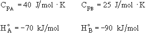
All heats of formation are referenced to 273K.
![]()
Solution
Mole Balances. Recalling Equation 8-XX and -rA = rB = rC
A:
![]()
B:
![]()
C:
![]()
Rate law
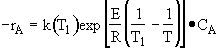
Stoichiometry
-rA = rB = rC
Flow: Laminar
Recalling the Energy Balance
![]()
Assumptions
Ur is virtually zero.
Neglect axial diffusion/dispersion flux w.r.t. convective flux
Neglect axial conduction w.r.t. axial convective
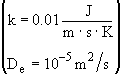
Let
![]()
![]()
Cooling jacket
![]()
Boundary conditions